Created by Yunhao Cao (Github@ToiletCommander) in Fall 2022 for UC Berkeley CS 285 (Sergey Levine).

Reference Notice: Material highly and mostly derived from Prof Levine's lecture slides, some ideas were borrowed from wikipedia & CS189.

This work is licensed under a Creative Commons Attribution-NonCommercial-ShareAlike 4.0 International License

General Introduction to RL (LEC 1)

Supervised ML

Given $D=\{(x_i,y_i)\}$

we will learn to predict $y$ from $x$.

usually assumes:

i.i.d. data (previous x,y pair does not affect next x, y pair)

known ground truth outputs in the training

Problem:

Cannot adapt if something fails.

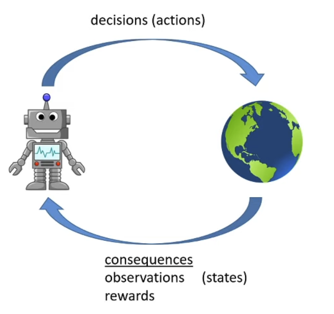
Reinforcement Learning:

Data is not i.i.d: previous outputs influence future inputs!

Ground truth answer is not known, only know if we succeeded or failed (but we generally know the reward)

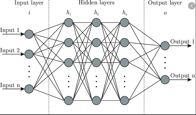
Compared to traditional reinforcement learning,

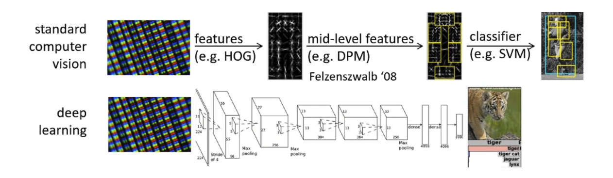
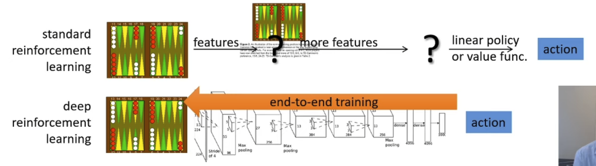
With DRL(Deep Reinforcement Learning), we can solve complex problems end-to-end!

But there are challenges:

1. Humans can learn incredibly quickly
   1. Deep RLs are usually slow
   2. probably because humans can reuse past knowledge

2. Not clear what the reward function should be

3. Not clear what the role of prediction should be

Types of RL Algorithms

Remember the objective of RL:

1. Policy Gradient
   1. Directly differentiate the above objective

2. Value-based
   1. Estimate value function or Q-function of the optimal policy (no explicit policy)
   2. Then use those functions to prove policy

3. Actor-critic (A mix between policy gradient and value-based)
   1. Estimate value function or Q-function of the current policy, use it to improve policy

4. Model-based RL
   1. Estimate the transition model, and then
      1. Use it for planning (no explicit policy)
      2. Use it to improve a policy
      3. Other variants

Supervised Learning of RL

Model-Based RL

e.g.

1. Dyna

2. Guided Policy Search

Generate samples(run the policy) ⇒

Fit a model of $p(s_{t+1}|s_t,a_t)$ ⇒

Then improve the policy(a few options)

Improving policy:

1. Just use the model to plan (no policy)
   1. Trajectory optimization / optimal control (primarily in continuous spaces)
      1. Backprop to optimize over actions
   2. Discrete planning in discrete action spaces
      1. Monte Carlo tree search

2. Backprop gradients into the policy
   1. Requires some tricks to make it work

3. Use the model to learn a separate value function or Q function
   1. Dynamic Programming
   2. Generate simulated experience for model-free learner

Value function based algorithms

e.g.

1. Q-Learning, DQN

2. Temporal Difference Learning

3. Fitted Value Iteration

Generate samples(run the policy) ⇒

Fit a model of $V(s)$ or $Q(s,a)$ ⇒

Then improve the policy(set $\pi(s) = \argmax_\theta Q(s,a)$)

Direct Policy Gradients

e.g.

1. REINFORCE Natural Policy Gradient

2. Trust Region Policy Optimization

Generate samples (run the policy) ⇒

Estimate the return

Improve the policy by

Actor-critic

e.g.

1. Asynchronous Advantage Actor-Critic (A3C)

2. Soft actor-critic (SAC)

Generate samples ⇒

Fit a model $V(s)$ or $Q(s,a)$ ⇒

Improve the policy

Tradeoff between algorithms

Sample efficiency

“How many samples for a good policy?”

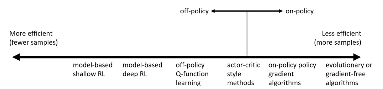
1. Most important question: Is the algorithm off-policy?
   1. Off policy means being able to improve the policy without generating new samples from that policy
   2. On policy means we need to generate new samples even if the policy is changed a little bit

Stability & Ease of use

1. Does our policy converge, and if it does, to what?

1. Value function fitting:
   1. Fixed point iteration
   2. At best, minimizes error of fit (“Bellman error”)
      1. Not the same as expected reward
   3. At worst, doesn’t optimize anything
      1. Many popular DRL value fitting algorithms are not guaranteed to converge to anything in the nonlinear case

2. Model-based RL
   1. Model is not optimized for expected reward
   2. Model minimizes error of fit
      1. This will converge
   3. No guarantee that better model = better policy

3. Policy Gradient
   1. The only one that performs Gradient Descent / Ascent on the true objective

Different assumptions

1. Stochastic or deterministic environments?

2. Continuous or discrete (states and action)?

3. Episodic(finite $T$) or infinite horizon?

4. Different things are easy or hard in different settings
   1. Easier to represent the policy?
   2. Easier to represent the model?

Common Assumptions:

1. Full observability
   1. Generally assumed by value function fitting methods
   2. Can be mitigated by adding recurrence

2. Episodic Learning
   1. Often assumed by pure policy gradient methods
   2. Assumed by some model-based RL methods
   3. Although other methods not assumed, tend to work better under this assumption

3. Continuity or smoothness
   1. Assumed by some continuous value function learning methods
   2. Often assumed by some model-based RL methods

Exploration

Offline RL (Batch RL / fully off-policy RL)

RL Theory

Variational Inference

No RL content in this chapter, but heavy links to RL algorithms

Control as an Inference Problem

Inverse Reinforcement Learning

Transfer Learning & Meta-Learning

Open Problems

Guest Lectures