∇θJ(θ)=Eτ∼pθ(τ)[(t=1∑T∇θlogπθ(at∣st))(t=1∑Tr(st,at))]≈N1i=1∑N(t=1∑T∇θlogπθ(ai,t∣si,t)(Reward to go Q^i,tt=1∑Tr(si,t,ai,t))
Q^i,t is the estimate of expected reward if we take action ai,t in state si,t
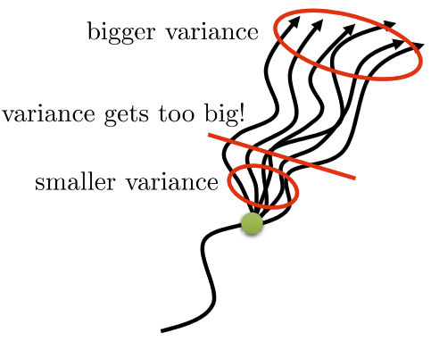
But Q^i,t currently has a very high variance
Q^i,t is only taking account of a specific chain of action-state pairs
This is because we approximated the gradient by stripping away the expectation
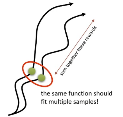
We can get a better estimate by using the true expected reward-to-go
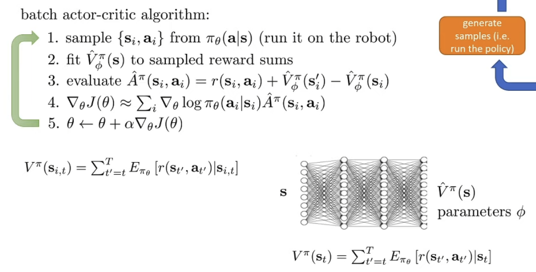
Qπ(st,at)=t′=t∑TEπθ[r(st′,at′)∣st,at]
What about baseline? Can we apply a baseline even if we have a true Q function?
Vπ(st)=Eat∼πθ(at∣st)[Qπ(st,at)]
Turns out that we can do better(less variance) than applying bt=N1∑iQ(si,t,ai,t) because with the value function, the baseline can be dependent on the state.
So now our gradient becomes
∇θJ(θ)≈N1i=1∑Nt=1∑T∇θlogπθ(ai,t∣si,t)How much better the action ai,t is than the average action(Qπ(si,t,ai,t)−Vπ(si,t))≈N1i=1∑Nt=1∑T∇θlogπθ(ai,t∣si,t)Aπ(si,t,ai,t)
We will also name something new: the advantage function:
How much better the action ai,t is than the average action
Aπ(st,at)=Qπ(st,at)−Vπ(st)
The better estimate Aπ estimate has, the lower variance ∇θJ(θ) has.
Lower variance than Monte Carlo evaluation, but higher bias (because V^ϕπ might be incorrect)
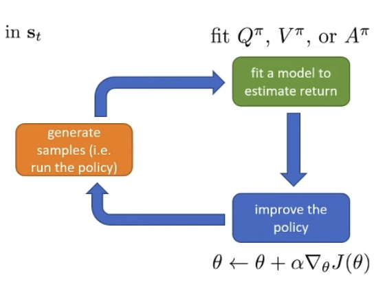
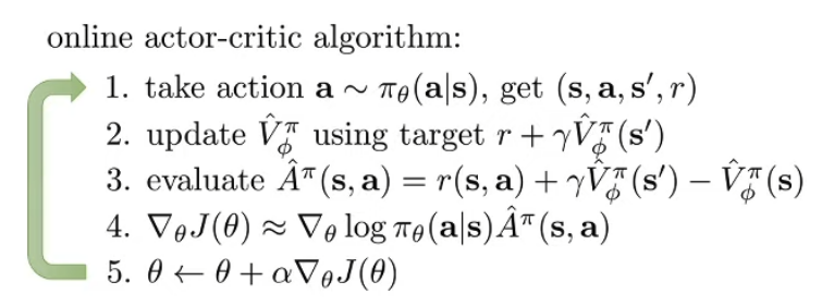
Batch actor-critic algorithm
⚠️
The fitted value function is not guarenteed to merge, same reason as the section “Value Function Learning Theory”
Discount Factor
If T→∞, V^ϕπ ⇒ the approximator for Vπ can get infinitely large in many cases, so we can regulate the reward to be “sooner rather than later”.
yi,t≈r(si,t,ai,t)+γV^ϕπ(si,t+1)
Where γ∈[0,1] is the discount factor, it let’s reward you get decay in every timestep ⇒ So that the obtainable reward in infinite lifetime can actually be bounded.
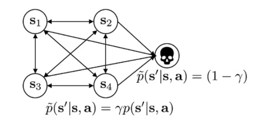
One understanding that γ affects policy is that γ adds a “death state” that once you’re in, you can never get out.
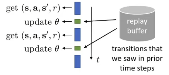
Idea: Collect data and instead of training on them directly, put them into a replay buffer. At training instead of using the data just collected, fetch one randomly from the replay buffer.
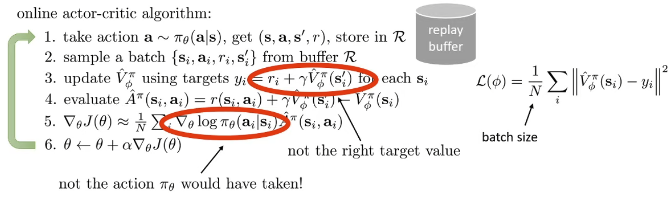
Coming from the online algorithm, let’s see what problems do we need to fix:
(1) Under current policy, it is possible that our policy would not even have taken the next action ai and therefore it’s not cool to assume we will arrive at the reward r(si,ai,si′) ⇒ We may not even arrive at state si’
(2) Same reason, we may not have taken ai as our action under the current policy
We can fix the problem in (1) by using Qπ(st,at) ⇒ replace the term γV^ϕπ(si’)
Now
L(ϕ)=N1i∑∣∣Q^ϕπ(si,ai)−yi)∣∣2
And we replace the target value
yi=ri+γQ^ϕπ(si′,this is sampled from current policy, ai′∼πθ(ai′π∣si′)ai′π)
Same for (2), sample an action from current policy aiπ∼πθ(ai∣si) rather than using the original data
It’s fine to have high variance (not being baselined), because it’s easier and now we don't need to generate more states ⇒ we can just generate more actions
In exchange use a larger batch size ⇒ all good!
🔥
Still one problem left ⇒ si did not come from pθ(s) ⇒ but nothing we can do
Not too bad ⇒ Initially we want optimal policy on pθ(s), but we actually get optimal policy on a broader distribution
Now our final result:
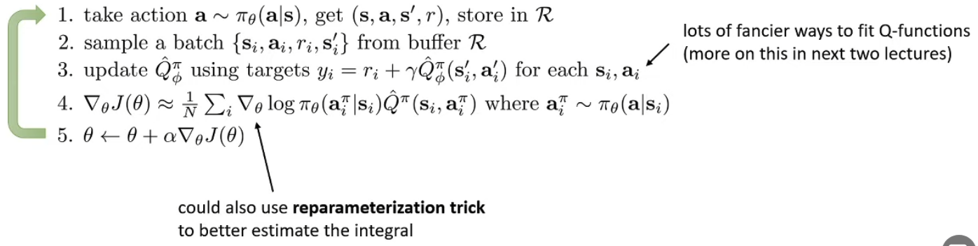
Example Practical Algorithm:
Tuomas Haarnoja, Aurick Zhou, Pieter Abbeel, Sergey Levine. Soft Actor-Critic: Off-Policy Maximum Entropy Deep Reinforcement Learning with a Stochastic Actor. 2018.
Not only does the policy gradient remain unbiased when you subtract any constant b, it still remains unbiased when you subtract any function that only depends on the state si (and not on the action)
Control variates - methods that use state and action dependent baselines
The n-step advantage estimator is good, but can we generalize(hybrid) it?
Instead of hard cutting between two estimators, why don’t we combine them everywhere?
A^GAEπ(st,at)=n=1∑∞wnA^nπ(st,at)
Where A^nπ stands for the n-step estimator
“Most prefer cutting earlier (less variance)”
So we set wn∝λn−1 ⇒ exponential falloff
Then
A^GAEπ(st,at)=t′=t∑∞(γλ)t′−tδt′, where δt′=r(st′,at′)+γV^ϕπ(st′+1)−V^ϕπ(st′)
🔥
Now we can just tradeoff the bias and variances using the parameter λ
Examples of actor-critic algorithms
Schulman, Moritz, Levine, Jordan, Abbeel ‘16. High dimensional continuous control with generalized advantage estimation
Batch-mode actor-critic
Blends Monte Carlo and GAE
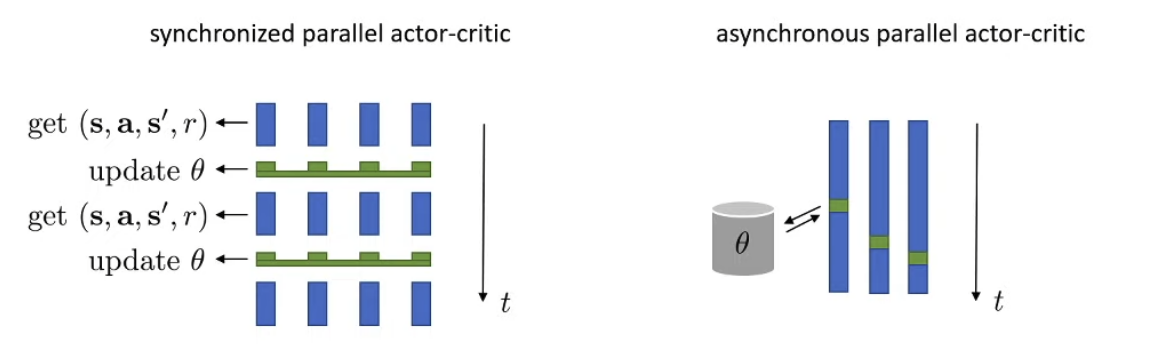
Mnih, Badia, Mirza, Graves, Lillicrap, Harley, Silver, Kavukcuoglu ‘16. Asynchronous methods for deep reinforcement learning
Online actor-critic, parallelized batch
CNN end-to-end
N-step returns with N=4
Single network for actor and critic
Suggested Readings
Classic: Sutton, McAllester, Singh, Mansour (1999). Policy gradient methods for reinforcement learning with function approximation: actor-critic algorithms with value function approximation
Talks about contents in this class
Mnih, Badia, Mirza, Graves, Lillicrap, Harley, Silver, Kavukcuoglu (2016). Asynchronous methods for deep reinforcement learning: A3C -- parallel online actor-critic
Schulman, Moritz, Levine, Jordan, Abbeel (2016). High-dimensional continuous control using generalized advantage estimation: batch-mode actor-critic with blended Monte Carlo and function approximator returns
Gu, Lillicrap, Ghahramani, Turner, Levine (2017). Q-Prop: sample-efficient policy-gradient with an off-policy critic: policy gradient with Q-function control variate