Does RL and optimal control provide a resonable model of human behavior?Is there a better explanation? Can we derive this porblem as probabilistic inference? How does it change our RL algorithms?
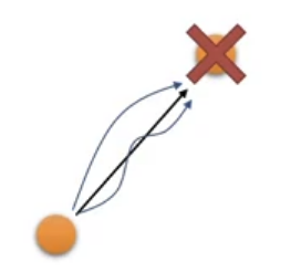
What if the data is not optimal? Humans (animals) make mistakes, but usually those mistakes still lead to a successful completion of taskSome mistakes matter more than others But good behavior is still the most likely Can we have a probabilistic model of good behavior?
We will introduce binary (True/False) Optimality Variables(O 1 , … , O T O_1, \dots, O_T O 1 , … , O T Is this person trying to be optimal at this point and time?
We will take this formula as given: (note that all of our rewards need to be negative)
Without loss of generality, just subtract reward by their maximum values. p ( O t ∣ s t , a t ) = exp ( r ( s t , a t ) ) p(O_t|s_t,a_t) = \exp(r(s_t,a_t)) p ( O t ∣ s t , a t ) = exp ( r ( s t , a t )) Then our probabilisitic model:
p ( τ undefined s 1 : T , a 1 : T ∣ O 1 : T ) = p ( τ , O 1 : T ) p ( O 1 : T ) ∝ p ( τ ) ∏ t exp ( r ( s t , a t ) ) = p ( τ ) exp ( ∑ t r ( s t , a t ) ) \begin{split}
p(\underbrace{\tau}_{\mathclap{s_{1:T},a_{1:T}}}|O_{1:T})
&= \frac{p(\tau, O_{1:T})}{p(O_{1:T})} \\
&\propto p(\tau) \prod_t \exp(r(s_t,a_t)) \\
&\quad = p(\tau) \exp(\sum_t r(s_t,a_t))
\end{split} p ( s 1 : T , a 1 : T τ ∣ O 1 : T ) = p ( O 1 : T ) p ( τ , O 1 : T ) ∝ p ( τ ) t ∏ exp ( r ( s t , a t )) = p ( τ ) exp ( t ∑ r ( s t , a t )) This can model suboptimal behavior (important for inverse RL) Can apply inference algorithms to solve control and planning problems Provides an explanation for why stochastic behavior might be preferred (useful for exploration and transfer learning) To do inference:
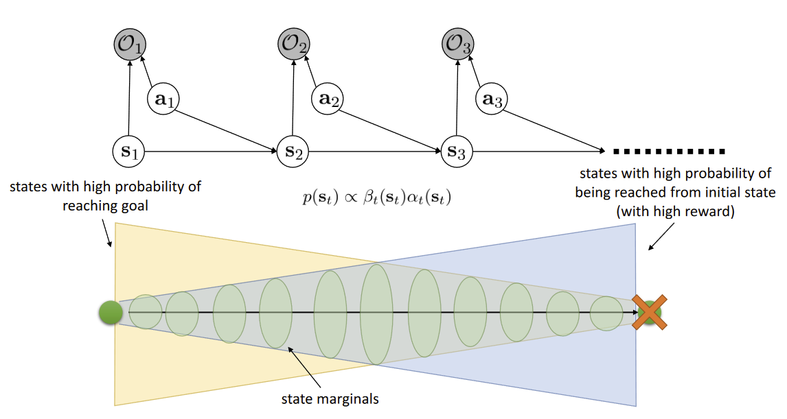
Compute backward messages β t ( s t , a t ) = p ( O t : T ∣ s t , a t ) \beta_t(s_t,a_t) = p(O_{t:T}|s_t,a_t) β t ( s t , a t ) = p ( O t : T ∣ s t , a t ) What’s the probability of being optimal from now until the end of the trajectory given the state and action we are in Compute policy p ( a t ∣ s t , O 1 : T ) p(a_t|s_t, O_{1:T}) p ( a t ∣ s t , O 1 : T ) Compute forward messages α t ( s t ) = p ( s t ∣ O 1 : t − 1 ) \alpha_t(s_t) = p(s_t | O_{1:t-1}) α t ( s t ) = p ( s t ∣ O 1 : t − 1 ) What’s the probability of being in state s t s_t s t
Backward Messages β t ( s t , a t ) = p ( O t : T ∣ s t , a t ) = ∫ p ( O t : T , s t + 1 ∣ s t , a t ) d s t + 1 = ∫ p ( O t + 1 : T ∣ s t + 1 ) p ( s t + 1 ∣ s t , a t ) p ( O t ∣ s t , a t ) d s t + 1 \begin{split}
\beta_t(s_t,a_t)
&= p(O_{t:T}|s_t,a_t) \\
&=\int p(O_{t:T},s_{t+1}|s_t,a_t) ds_{t+1} \\
&=\int p(O_{t+1:T}|s_{t+1}) p(s_{t+1}|s_t,a_t) p(O_t|s_t, a_t) ds_{t+1} \\
\end{split} β t ( s t , a t ) = p ( O t : T ∣ s t , a t ) = ∫ p ( O t : T , s t + 1 ∣ s t , a t ) d s t + 1 = ∫ p ( O t + 1 : T ∣ s t + 1 ) p ( s t + 1 ∣ s t , a t ) p ( O t ∣ s t , a t ) d s t + 1 Note:
p ( O t + 1 ∣ s t + 1 ) = ∫ p ( O t + 1 : T ∣ s t + 1 , a t + 1 ) undefined β t + 1 ( s t + 1 , a t + 1 ) p ( a t + 1 ∣ s t + 1 ) undefined which actions are likely a priori d a t + 1 p(O_{t+1}|s_{t+1}) = \int \underbrace{p(O_{t+1:T}|s_{t+1}, a_{t+1})}_{\beta_{t+1}(s_{t+1},a_{t+1})} \underbrace{p(a_{t+1}|s_{t+1})}_{\text{which actions are likely a priori}} da_{t+1} p ( O t + 1 ∣ s t + 1 ) = ∫ β t + 1 ( s t + 1 , a t + 1 ) p ( O t + 1 : T ∣ s t + 1 , a t + 1 ) which actions are likely a priori p ( a t + 1 ∣ s t + 1 ) d a t + 1 p ( a t + 1 ∣ s t + 1 ) p(a_{t+1}|s_{t+1}) p ( a t + 1 ∣ s t + 1 ) We will assume uniform for now
Reasonable because:
Don’t know anything about the policy, reasonable to assume uniform Can modify reward function later to impose non-uniformity Action Prior in Backward Pass of Control as Inference in RL (1) Therefore,
β t ( s t , a t ) = ∫ p ( O t + 1 : T ∣ s t + 1 ) p ( s t + 1 ∣ s t , a t ) p ( O t ∣ s t , a t ) d s t + 1 = p ( O t ∣ s t , a t ) E s t + 1 ∣ s t , a t [ β t + 1 ( s t + 1 ) undefined = E a t ∼ p ( a t ∣ s t ) [ β t ( s t , a t ) ] ] \begin{split}
\beta_t(s_t,a_t)
&=\int p(O_{t+1:T}|s_{t+1}) p(s_{t+1}|s_t,a_t) p(O_t|s_t, a_t) ds_{t+1} \\
&=p(O_t|s_t,a_t) \mathbb{E}_{s_{t+1}|s_t,a_t}[\underbrace{\beta_{t+1}(s_{t+1})}_{\mathclap{=\mathbb{E}_{a_t \sim p(a_t | s_t)}[\beta_t (s_t,a_t)]}}]
\end{split} β t ( s t , a t ) = ∫ p ( O t + 1 : T ∣ s t + 1 ) p ( s t + 1 ∣ s t , a t ) p ( O t ∣ s t , a t ) d s t + 1 = p ( O t ∣ s t , a t ) E s t + 1 ∣ s t , a t [ = E a t ∼ p ( a t ∣ s t ) [ β t ( s t , a t )] β t + 1 ( s t + 1 ) ] This algorithm is called the backward pass β \beta β t = T − 1 t=T-1 t = T − 1 1 1 1
We will take a closer look at the backward pass
Let V t ( s t ) = log β t ( s t ) V_t(s_t) = \log \beta_t(s_t) V t ( s t ) = log β t ( s t ) Q t ( s t , a t ) = log β t ( s t , a t ) Q_t (s_t, a_t) = \log \beta_t(s_t,a_t) Q t ( s t , a t ) = log β t ( s t , a t )
V t ( s t ) = log ∫ exp ( Q t ( s t , a t ) ) d a t V_t(s_t) = \log \int \exp(Q_t(s_t,a_t)) da_t V t ( s t ) = log ∫ exp ( Q t ( s t , a t )) d a t We see that V t ( s t ) → max a t Q t ( s t , a t ) V_t(s_t) \to \max_{a_t} Q_t(s_t,a_t) V t ( s t ) → max a t Q t ( s t , a t ) Q t ( s t , a t ) Q_t(s_t,a_t) Q t ( s t , a t ) soft relaxation of the max operator )
Let’s also evaluate Q t Q_t Q t
Q t ( s t , a t ) = r ( s t , a t ) + log E [ exp ( V t + 1 ( s t + 1 ) ) ] Q_t(s_t,a_t) = r(s_t,a_t) + \log \mathbb{E}[\exp(V_{t+1}(s_{t+1}))] Q t ( s t , a t ) = r ( s t , a t ) + log E [ exp ( V t + 1 ( s t + 1 ))] If we have determinimistic transition, then the update of this Q t Q_t Q t
Q t ( s t , a t ) = r ( s t , a t ) + V t + 1 ( s t + 1 ) Q_t(s_t,a_t) = r(s_t,a_t) + V_{t+1}(s_{t+1}) Q t ( s t , a t ) = r ( s t , a t ) + V t + 1 ( s t + 1 ) But if we have non-deterministic transitions,. then this update of Q t Q_t Q t will lead to optimistic transitions dominating the update
The reason we got this is because when we ask the optimality variable “How optimal are we at the time step”We are not differentiating between if we’re optimal because we got a lucky transition or if we performed the optimal action
Policy Computation Policy ⇒ p ( a t ∣ s t , O 1 : T ) p(a_t|s_t, O_{1:T}) p ( a t ∣ s t , O 1 : T )
p ( a t ∣ s t , O 1 : T ) = π ( a t ∣ s t ) = p ( a t ∣ s t , O t : T ) = p ( a t , s t ∣ O t : T ) p ( s t ∣ O t : T ) = p ( O t : T ∣ a t , s t ) p ( a t , s t ) / p ( O t : T ) p ( O t : T ∣ s t ) p ( s t ) / p ( O t : T ) = p ( O t : T ∣ s t , a t ) p ( O t : T ∣ s t ) p ( a t , s t ) p ( s t ) = β t ( s t , a t ) β t ( s t ) p ( a t ∣ s t ) undefined action prior assumed to be uniform = exp ( Q t ( s t , a − t ) − V t ( s t ) ) = exp ( A t ( s t , a t ) ) ≈ exp ( 1 α undefined α is the added temperature A t ( s t , a t ) ) \begin{split}
p(a_t|s_t,O_{1:T})
&= \pi(a_t|s_t) \\
&=p(a_t|s_t,O_{t:T}) \\
&= \frac{p(a_t,s_t|O_{t:T})}{p(s_t|O_{t:T})} \\
&=\frac{p(O_{t:T}|a_t,s_t) p(a_t,s_t)/p(O_{t:T})}{p(O_{t:T}|s_t) p(s_t) / p(O_{t:T})} \\
&=\frac{p(O_{t:T}|s_t,a_t)}{p(O_{t:T}|s_t)} \frac{p(a_t,s_t)}{p(s_t)} \\
&=\frac{\beta_t(s_t,a_t)}{\beta_t(s_t)} \underbrace{p(a_t|s_t)}_{\mathclap{\text{action prior assumed to be uniform}}} \\
&=\exp(Q_t(s_t,a-t) - V_t(s_t)) = \exp(A_t(s_t,a_t)) \\
&\approx \exp(\underbrace{\frac{1}{\alpha}}_{\mathclap{\text{$\alpha$ is the added temperature}}}A_t(s_t,a_t))
\end{split} p ( a t ∣ s t , O 1 : T ) = π ( a t ∣ s t ) = p ( a t ∣ s t , O t : T ) = p ( s t ∣ O t : T ) p ( a t , s t ∣ O t : T ) = p ( O t : T ∣ s t ) p ( s t ) / p ( O t : T ) p ( O t : T ∣ a t , s t ) p ( a t , s t ) / p ( O t : T ) = p ( O t : T ∣ s t ) p ( O t : T ∣ s t , a t ) p ( s t ) p ( a t , s t ) = β t ( s t ) β t ( s t , a t ) action prior assumed to be uniform p ( a t ∣ s t ) = exp ( Q t ( s t , a − t ) − V t ( s t )) = exp ( A t ( s t , a t )) ≈ exp ( α is the added temperature α 1 A t ( s t , a t )) Natural interpretation:better actions are more probable Analogous to Boltzmann exploration Approaches greedy policy as temperature decreases
Forward Messages α t ( s t ) = p ( s t ∣ O 1 : t − 1 ) = ∫ p ( s t , s t − 1 , a t − 1 ∣ O 1 : t − 1 ) d s t − 1 d a t − 1 = ∫ p ( s t ∣ s t − 1 , a t − 1 , O 1 : t − 1 ) p ( a t − 1 ∣ s t − 1 , O 1 : t − 1 ) p ( s t − 1 ∣ O 1 : t − 1 ) d s t − 1 d a t − 1 = ∫ p ( s t ∣ s t − 1 , a t − 1 ) p ( a t − 1 ∣ s t − 1 , O 1 : t − 1 ) p ( s t − 1 ∣ O 1 : t − 1 ) d s t − 1 d a t − 1 \begin{split}
\alpha_t(s_t)
&= p(s_t|O_{1:t-1}) \\
&=\int p(s_t,s_{t-1},a_{t-1}|O_{1:t-1}) ds_{t-1}da_{t-1} \\
&=\int p(s_t|s_{t-1},a_{t-1}, O_{1:t-1}) p(a_{t-1}|s_{t-1},O_{1:t-1}) p(s_{t-1}|O_{1:t-1}) ds_{t-1} da_{t-1} \\
&= \int p(s_t | s_{t-1}, a_{t-1})p(a_{t-1}|s_{t-1},O_{1:t-1}) p(s_{t-1}|O_{1:t-1}) ds_{t-1} da_{t-1} \\
\end{split} α t ( s t ) = p ( s t ∣ O 1 : t − 1 ) = ∫ p ( s t , s t − 1 , a t − 1 ∣ O 1 : t − 1 ) d s t − 1 d a t − 1 = ∫ p ( s t ∣ s t − 1 , a t − 1 , O 1 : t − 1 ) p ( a t − 1 ∣ s t − 1 , O 1 : t − 1 ) p ( s t − 1 ∣ O 1 : t − 1 ) d s t − 1 d a t − 1 = ∫ p ( s t ∣ s t − 1 , a t − 1 ) p ( a t − 1 ∣ s t − 1 , O 1 : t − 1 ) p ( s t − 1 ∣ O 1 : t − 1 ) d s t − 1 d a t − 1 Note:
p ( a t − 1 ∣ s t − 1 , O t − 1 ) p ( s t − 1 ∣ O 1 : t − 1 ) = p ( O t − 1 ∣ s t − 1 , a t − 1 ) p ( a t − 1 ∣ s t − 1 ) undefined uniform p ( O t − 1 ∣ s t − 1 ) p ( O t − 1 ∣ s t − 1 ) p ( s t − 1 ∣ O 1 : t − 2 ) undefined α t − 1 ( s t − 1 ) p ( O t − 1 ∣ O 1 : t − 2 ) = p ( O t − 1 ∣ s t − 1 , a t − 1 ) p ( O t − 1 ∣ O 1 : t − 2 ) α t − 1 ( s t − 1 ) \begin{split}
p(a_{t-1}|s_{t-1}, O_{t-1}) p(s_{t-1}|O_{1:t-1})
&= \frac{p(O_{t-1}|s_{t-1},a_{t-1})\overbrace{p(a_{t-1}|s_{t-1})}^{\text{uniform}}}{p(O_{t-1}|s_{t-1})} \frac{p(O_{t-1}|s_{t-1}) \overbrace{p(s_{t-1}|O_{1:t-2})}^{\alpha_{t-1}(s_{t-1})}}{p(O_{t-1}|O_{1:t-2})} \\
&=\frac{p(O_{t-1}|s_{t-1},a_{t-1})}{p(O_{t-1}|O_{1:t-2})} \alpha_{t-1}(s_{t-1})
\end{split} p ( a t − 1 ∣ s t − 1 , O t − 1 ) p ( s t − 1 ∣ O 1 : t − 1 ) = p ( O t − 1 ∣ s t − 1 ) p ( O t − 1 ∣ s t − 1 , a t − 1 ) p ( a t − 1 ∣ s t − 1 ) uniform p ( O t − 1 ∣ O 1 : t − 2 ) p ( O t − 1 ∣ s t − 1 ) p ( s t − 1 ∣ O 1 : t − 2 ) α t − 1 ( s t − 1 ) = p ( O t − 1 ∣ O 1 : t − 2 ) p ( O t − 1 ∣ s t − 1 , a t − 1 ) α t − 1 ( s t − 1 ) What if we want to know p ( s t ∣ O 1 : T ) p(s_t|O_{1:T}) p ( s t ∣ O 1 : T )
p ( s t ∣ O 1 : T ) = p ( s t , O 1 : T ) p ( O 1 : T ) = p ( O t : T ∣ s t ) undefined β t ( s t ) p ( s t , O 1 : t − 1 ) p ( O 1 : T ) ∝ β t ( s t ) p ( s t ∣ O 1 : t − 1 ) p ( O 1 : t − 1 ) ∝ β t ( s t ) α t ( s t ) \begin{split}
p(s_t|O_{1:T})
&= \frac{p(s_t,O_{1:T})}{p(O_1:T)} \\
&= \frac{\overbrace{p(O_{t:T}|s_t)}^{\beta_t(s_t)} p(s_t, O_{1:t-1})}{p(O_{1:T})} \\
&\propto \beta_t(s_t) p(s_t|O_{1:t-1})p(O_{1:t-1}) \\
&\propto \beta_t(s_t) \alpha_t(s_t)
\end{split} p ( s t ∣ O 1 : T ) = p ( O 1 : T ) p ( s t , O 1 : T ) = p ( O 1 : T ) p ( O t : T ∣ s t ) β t ( s t ) p ( s t , O 1 : t − 1 ) ∝ β t ( s t ) p ( s t ∣ O 1 : t − 1 ) p ( O 1 : t − 1 ) ∝ β t ( s t ) α t ( s t ) Yellow cone shape is the beta, blue cone is the alpha
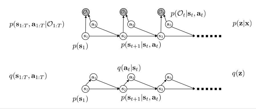
Control as Variational Inference In continuous high-dimensional spaces we have to approximate Inference problem:
p ( s 1 : T , a 1 : T ∣ O 1 : T ) p(s_{1:T}, a_{1:T}|O_{1:T}) p ( s 1 : T , a 1 : T ∣ O 1 : T ) Marginalizing and conditioning, we get the policy
π ( a t ∣ s t ) = p ( a t ∣ s t , O 1 : T ) \pi(a_t|s_t) = p(a_t|s_t,O_{1:T}) π ( a t ∣ s t ) = p ( a t ∣ s t , O 1 : T ) However,
p ( s t + 1 ∣ s t , a t , O 1 : T ) ≠ p ( s t + 1 ∣ s t , a t ) p(s_{t+1}|s_t,a_t,O_{1:T}) \ne p(s_{t+1}|s_t,a_t) p ( s t + 1 ∣ s t , a t , O 1 : T ) = p ( s t + 1 ∣ s t , a t ) Instead of asking
“Given that you obtained high reward, what was your action probability and your transition probability” We want to ask
“Given that you obtained high reward, what was your action probability given that your transition probability did not change ❓
Can we find another distribution
q ( s 1 : T , a 1 : T ) q(s_{1:T}, a_{1:T}) q ( s 1 : T , a 1 : T ) that is close to
p ( s 1 : T , a 1 : T ∣ O 1 : T ) p(s_{1:T}, a_{1:T}|O_{1:T}) p ( s 1 : T , a 1 : T ∣ O 1 : T ) but has dynamics
p ( s t + 1 ∣ s t , a t ) p(s_{t+1}|s_t,a_t) p ( s t + 1 ∣ s t , a t ) ?
Let’s try variational inference!
Let q ( s 1 : T , a 1 : T ) = p ( s 1 ) ∏ t p ( s t + 1 ∣ s t , a t ) q ( a t ∣ s t ) q(s_{1:T}, a_{1:T}) = p(s_1) \prod_{t} p(s_{t+1}|s_t,a_t) q(a_t | s_t) q ( s 1 : T , a 1 : T ) = p ( s 1 ) ∏ t p ( s t + 1 ∣ s t , a t ) q ( a t ∣ s t )
Let x = O 1 : T , z = ( s 1 : T , a 1 : T ) x = O_{1:T}, z = (s_{1:T}, a_{1:T}) x = O 1 : T , z = ( s 1 : T , a 1 : T )
The variational lower bound
log p ( x ) ≥ E z ∼ q ( z ) [ log p ( x , z ) − log q ( z ) ] \log p(x) \ge \mathbb{E}_{z \sim q(z)}[\log p(x,z) - \log q(z)] log p ( x ) ≥ E z ∼ q ( z ) [ log p ( x , z ) − log q ( z )] Substituting in our definitions,
log p ( O 1 : T ) ≥ E ( s 1 : T , a 1 : T ) ∼ q [ log p ( s 1 ) + ∑ t = 1 T log p ( s t + 1 ∣ s t , a t ) + ∑ t = 1 T log p ( O t ∣ s t , a t ) − log p ( s 1 ) − ∑ t = 1 T log p ( s t + 1 ∣ s t , a t ) − ∑ t = 1 T log q ( a t ∣ s t ) ] = E ( s 1 : T , a 1 : T ) ∼ q [ ∑ t r ( s t , a t ) − log q ( a t ∣ s t ) ] = ∑ t E ( s t , a t ) ∼ q [ r ( s t , a t ) + H ( q ( a t ∣ s t ) ) ] \begin{split}
\log p(O_{1:T})
\ge &\mathbb{E}_{(s_{1:T}, a_{1:T}) \sim q}[\log p(s_1) + \sum_{t=1}^T \log p(s_{t+1}|s_t,a_t) + \sum_{t=1}^T \log p(O_t|s_t,a_t) \\
&-\log p(s_1) - \sum_{t=1}^T \log p(s_{t+1}|s_t, a_t) - \sum_{t=1}^T \log q(a_t|s_t)] \\
&= \mathbb{E}_{(s_{1:T}, a_{1:T}) \sim q}[\sum_t r(s_t, a_t) - \log q(a_t|s_t)] \\
&= \sum_t \mathbb{E}_{(s_t,a_t) \sim q}[r(s_t,a_t) + H(q(a_t|s_t))]
\end{split} log p ( O 1 : T ) ≥ E ( s 1 : T , a 1 : T ) ∼ q [ log p ( s 1 ) + t = 1 ∑ T log p ( s t + 1 ∣ s t , a t ) + t = 1 ∑ T log p ( O t ∣ s t , a t ) − log p ( s 1 ) − t = 1 ∑ T log p ( s t + 1 ∣ s t , a t ) − t = 1 ∑ T log q ( a t ∣ s t )] = E ( s 1 : T , a 1 : T ) ∼ q [ t ∑ r ( s t , a t ) − log q ( a t ∣ s t )] = t ∑ E ( s t , a t ) ∼ q [ r ( s t , a t ) + H ( q ( a t ∣ s t ))] ⇒ maximize reward and maximize action entropy!
Optimize Variational Lower Bound Base case: Solve for q ( a T ∣ s T ) q(a_T|s_T) q ( a T ∣ s T )
q ( a T ∣ s T ) = arg max E s T ∼ q ( s T ) [ E a T ∼ q ( a T ∣ s T ) [ r ( s T , a T ) ] + H ( q ( a T ∣ s T ) ) ] = arg max E s T ∼ q ( s T ) [ E a T ∼ q ( a T ∣ s T ) [ r ( s T , a T ) − log q ( a T ∣ s T ) ] ] \begin{split}
q(a_T|s_T)
&= \argmax \mathbb{E}_{s_T \sim q(s_T)}[\mathbb{E}_{a_T \sim q(a_T|s_T)}[r(s_T, a_T)] + H(q(a_T|s_T))] \\
&= \argmax \mathbb{E}_{s_T \sim q(s_T)}[\mathbb{E}_{a_T \sim q(a_T|s_T)}[r(s_T, a_T) - \log q(a_T|s_T)]]
\end{split} q ( a T ∣ s T ) = arg max E s T ∼ q ( s T ) [ E a T ∼ q ( a T ∣ s T ) [ r ( s T , a T )] + H ( q ( a T ∣ s T ))] = arg max E s T ∼ q ( s T ) [ E a T ∼ q ( a T ∣ s T ) [ r ( s T , a T ) − log q ( a T ∣ s T )]] optimized when q ( a T ∣ s T ) ∝ exp ( r ( s T , a T ) ) q(a_T|s_T) \propto \exp(r(s_T,a_T)) q ( a T ∣ s T ) ∝ exp ( r ( s T , a T ))
q ( a T ∣ s T ) = exp ( r ( s T , a T ) ) ∫ exp ( r ( s T , a ) ) d a = exp ( Q ( s T , a T ) − V ( s T ) ) q(a_T|s_T) = \frac{\exp(r(s_T,a_T))}{\int \exp(r(s_T, a)) da} = \exp(Q(s_T,a_T) - V(s_T)) q ( a T ∣ s T ) = ∫ exp ( r ( s T , a )) d a exp ( r ( s T , a T )) = exp ( Q ( s T , a T ) − V ( s T )) V ( s T ) = log ∫ exp ( Q ( s T , a T ) ) d a T V(s_T) = \log \int \exp(Q(s_T,a_T)) da_T V ( s T ) = log ∫ exp ( Q ( s T , a T )) d a T Therefore
E s T ∼ q ( s T ) [ E a T ∼ q ( a T ∣ s T ) [ r ( s T , a T ) − log q ( a T ∣ s T ) ] ] = E s T ∼ q ( s T ) [ E a T ∼ q ( a T ∣ s T ) [ V ( s T ) ] ] \mathbb{E}_{s_T \sim q(s_T)}[\mathbb{E}_{a_T \sim q(a_T|s_T)}[r(s_T, a_T) - \log q(a_T|s_T)]] = \mathbb{E}_{s_T \sim q(s_T)}[\mathbb{E}_{a_T \sim q(a_T|s_T)}[V(s_T)]] E s T ∼ q ( s T ) [ E a T ∼ q ( a T ∣ s T ) [ r ( s T , a T ) − log q ( a T ∣ s T )]] = E s T ∼ q ( s T ) [ E a T ∼ q ( a T ∣ s T ) [ V ( s T )]] ⚠️
Dynamic Programming Solution!
Levine (2018). Reinforcement Learning and Control as Probabilistic Inference
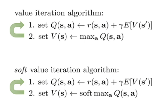
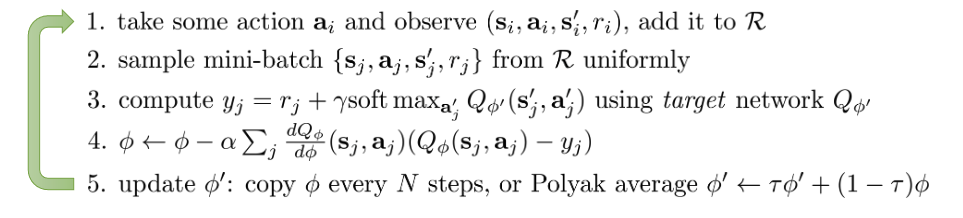
Q-Learning with softoptimality Standard Q-Learning:
ϕ ← ϕ + α ∇ ϕ Q ϕ ( s , a ) ( r ( s , a ) + γ V ( s ′ ) − Q ϕ ( s , a ) ) \phi \leftarrow \phi + \alpha \nabla_\phi Q_\phi(s,a)(r(s,a) + \gamma V(s') - Q_\phi(s,a)) ϕ ← ϕ + α ∇ ϕ Q ϕ ( s , a ) ( r ( s , a ) + γV ( s ′ ) − Q ϕ ( s , a )) Standard Q-Learning Target
V ( s ′ ) = max a ′ Q ϕ ( s ′ , a ′ ) V(s') = \max_{a'} Q_\phi(s',a') V ( s ′ ) = a ′ max Q ϕ ( s ′ , a ′ ) Soft Q-Learning
ϕ ← ϕ + α ∇ ϕ Q ϕ ( s , a ) ( r ( s , a ) + γ V ( s ′ ) − Q ϕ ( s , a ) ) \phi \leftarrow \phi + \alpha \nabla_{\phi} Q_\phi(s,a)(r(s,a) + \gamma V(s') - Q_\phi(s,a)) ϕ ← ϕ + α ∇ ϕ Q ϕ ( s , a ) ( r ( s , a ) + γV ( s ′ ) − Q ϕ ( s , a )) Soft Q-Learning Target
V ( s ′ ) = soft max a ′ Q ϕ ( s ′ , a ′ ) = log ∫ exp ( Q ϕ ( s ′ , a ′ ) ) d a ′ V(s') = \text{soft max}_{a'} Q_\phi(s',a') = \log \int \exp (Q_\phi(s',a')) da' V ( s ′ ) = soft max a ′ Q ϕ ( s ′ , a ′ ) = log ∫ exp ( Q ϕ ( s ′ , a ′ )) d a ′ Policy
π ( a ∣ s ) = exp ( Q ϕ ( s , a ) − V ( s ) ) = exp ( A ( s , a ) ) \pi(a|s) = \exp(Q_\phi(s,a) - V(s)) = \exp(A(s,a)) π ( a ∣ s ) = exp ( Q ϕ ( s , a ) − V ( s )) = exp ( A ( s , a ))
Policy Gradient with Soft Optimality (”Entropy regularized” policy gradient) π ( a ∣ s ) = exp ( Q ϕ ( s , a ) − V ( s ) ) \pi(a|s) = \exp(Q_\phi(s,a) - V(s)) π ( a ∣ s ) = exp ( Q ϕ ( s , a ) − V ( s )) this policy optimizes ∑ t E π ( s t , a t ) [ r ( s t , a t ) ] + E π ( s t ) [ H ( π ( a t ∣ s t ) ) ] \sum_t \mathbb{E}_{\pi(s_t,a_t)}[r(s_t, a_t)] + \mathbb{E}_{\pi(s_t)}[H(\pi(a_t|s_t))] ∑ t E π ( s t , a t ) [ r ( s t , a t )] + E π ( s t ) [ H ( π ( a t ∣ s t ))]
Intuition:
π ( a ∣ s ) ∝ exp ( Q ϕ ( s , a ) ) \pi(a|s) \propto \exp(Q_\phi(s,a)) π ( a ∣ s ) ∝ exp ( Q ϕ ( s , a )) π \pi π D K L ( π ( a ∣ s ) ∣ ∣ 1 Z exp ( Q ( s , a ) ) ) D_{KL}(\pi(a|s) || \frac{1}{Z} \exp(Q(s,a))) D K L ( π ( a ∣ s ) ∣∣ Z 1 exp ( Q ( s , a ))) D K L ( π ( a ∣ s ) ∣ ∣ 1 Z exp ( Q ( s , a ) ) ) = E π ( a ∣ s ) [ Q ( s , a ) ] − H ( π ) D_{KL}(\pi(a|s) || \frac{1}{Z} \exp(Q(s,a))) = \mathbb{E}_{\pi(a|s)} [Q(s,a) ] - H(\pi) D K L ( π ( a ∣ s ) ∣∣ Z 1 exp ( Q ( s , a ))) = E π ( a ∣ s ) [ Q ( s , a )] − H ( π ) Combats premature entropy collapse
Benefits of soft optimality Improve exploration and prevent entropy collapse Easier to specialize (finetune) policies for more speicific tasks Principled approach to break ties Better robustness (due to wider coverage of states) Can reduce to hard optimality as reward magnitude increases Good model for modeling human behavior
Suggested Readings (Soft Optimality) Todorov. (2006). Linearly solvable Markov decision problems: one framework for reasoning about soft optimality. Todorov. (2008). General duality between optimal control and estimation: primer on the equivalence between inference and control. Kappen. (2009). Optimal control as a graphical model inference problem: frames control as an inference problem in a graphical model. Ziebart. (2010). Modeling interaction via the principle of maximal causal entropy: connection between soft optimality and maximum entropy modeling. Rawlik, Toussaint, Vijaykumar. (2013). On stochastic optimal control and reinforcement learning by approximate inference: temporal difference style algorithm with soft optimality. Haarnoja*, Tang*, Abbeel, L. (2017). Reinforcement learning with deep energy based models: soft Q-learning algorithm, deep RL with continuous actions and soft optimality Nachum, Norouzi, Xu, Schuurmans. (2017). Bridging the gap between value and policy based reinforcement learning. Schulman, Abbeel, Chen. (2017). Equivalence between policy gradients and soft Q-learning. Haarnoja, Zhou, Abbeel, L. (2018). Soft Actor-Critic: Off-Policy Maximum Entropy Deep Reinforcement Learning with a Stochastic Actor. Levine. (2018). Reinforcement Learning and Control as Probabilistic Inference: Tutorial and Review