Exploration
Exploration (Lec 13)
It’s hard for algorithms to know what rules of the environment are “Mao” Game
- The only rule you may be told is this one
- Incur a penalty when you break a rule
- Can only discover rules through trial and error
- Rules don’t always make sense to you
So here is the definition of exploration problem:
- How can an agent discover high-reward strategies that require a temporally extended sequence of complex behaviors that, individually, are not rewarding?
- How can an agent decide whether to attempt new behaviors or continue to do best things it knows so far?
So can we derive an optimal exploration strategy:
Tractable(易于理解) - If it is easy to know that the policy is optimal or not
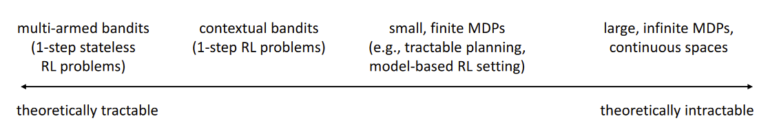
- Multi-arm bandits (1-step, stateless RL) / Contextual bandits (1 step, but there’s a state)
- Can formalize exploration as POMDP(Partial-observed MDP because although there’s only one time, performing actions help us expand our knowledge) identification
- policy learning is trivial even with POMDP
- small, finite MDPs
- Can frame as Bayesian model identification, reason explicitly about value of information
- Large or infinite MDPs
- Optimal methods don’t work
- Exploring with random actions: oscillate back and forth, might not go to a coherent or interesting place
- But can take inspiration from optimal methods in smaller settings
- use hacks
- Optimal methods don’t work
Bandits
The dropsophila(黑腹果蝇, 模式生物) of exploration problems
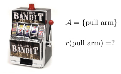
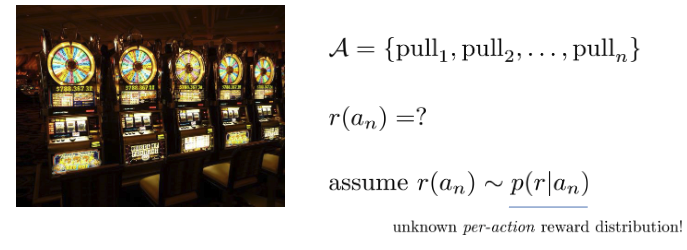
So the definition of the bandit:
Assume
e.g. and
Where (but you don’t know):
This defines a POMDP with
Belief state is
Solving the POMDP yields the optimal exploration strategy
But this is an overkill - belief state is huge! ⇒ we can do very well with much simpler strategies
We will define regret as the difference from optimal policy at time step
How do we beat bandit?
- Variety of relatively simple strategies
- Often can provide theoretical guarantees on regret
- Empirical performance may vary
- Exploration strategies for more complex MDP domains will be inmspired by those strategies
Optimistic exploration
- Keep track of average reward for each action a
- Exploitation: pick
- Optimistic Estimate:
- “Try each arm until you are sure it’s not great”
- where is number of times we have picked this action
To put this in practice, use ⇒ easy to add in but hard to tune the weights of .
Problem is in continuous states ⇒ we never see same thing twice ⇒ but some states are more similar than others
Beliemare et al. “Unifying Count-based Exploration …”
So we will
- Fit a density model or
- might be high even for a new if is similar to previous seen states
- But how can the distribution of match the distribution of a count?
Notice that the true probability is , and after seeing ,
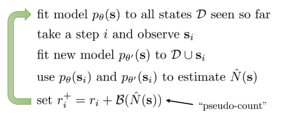
How to get to ?
Solving the equation, we find
Different classes of bonuses:
- UCB bonus
- MBIE-EB (Strehl & Littman, 2008):
- BEB (Kolter & Ng, 2009):
So we need to output densities, but doesn’t necessarily need to produce great samples
Opposite considerations from many popular generative models like GANs
Bellemare et al. “CTS” Model: Condition each pixel on its top-left neighborhood
Other models: Stochastic neural networks, compression length, EX2
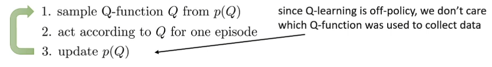
Probability Matching / Posterior Sampling (Thompson Sampling)
Assume ⇒ which defines a POMDP with
Belief state is
Idea:
- Sample
- Pretend the model is correct
- Take the optimal action
- Update the model
Chapelle & Li, “An Empirical Evaluation of Thompson Sampling.”
⇒ Hard to analyze theoretically but can work very well empirically
Osband et al. “Deep Exploration via Boostrapped DQN”
- What do we sample?
- how do we represent the distribution?
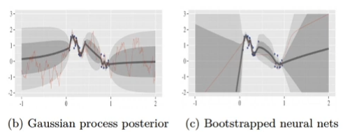
Bootstrap ensembles:
- Given a dataset , resample with replacement times to get
- train each model on
- To sample from , sample and use
- No change to original reward function
- Very good bonuses often do better than this
Methods that use Information Gain
Bayesian Experimental Design
If we want to determine some latent variable ⇒ might be optimal action or its value
Which action do we take?
Let be the current entropy of our estimate
Let be the entropy of our estimate after observation ( might be in the case of RL)
The lower the entropy, the more precisely we know
Typically depends on action, so we will use the notion
Russo & Van Roy “Learning to Optimize via Information-Directed Sampling”
Observe reward and learn parameters of
We want to gain more information but we don’t want our policy to be suboptimal
So we will choose according to
Houthooft et al. “VIME”
Question:
- Information gain about what?
- Reward
- Not useful as reward is sparse
- State density
- A bit strange, but somewhat makes sense!
- Dynamics
- Good proxy for learning the MDP, though still heuristic
- Reward
Generally they are intractable to use exactly, regardless of what is being estimated
A few approximations:
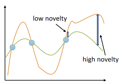
- Prediction Gain (Schmidhuber ‘91, Bellemare ‘16)
-
- If density changed a lot, then the state is novel
- Variational Inference (Houthooft et al. “VIME”)
- IG can be equivalently written as
- Learn about transitions
-
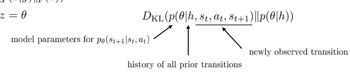
- Intuition: a transition is more informative if it causes belief over to change
- Idea:
- Use variational inference to estimate
- Specifically optimize variational lower bound
- Represent as product of independent Gaussian parameter distributions with mean
-
-
- See Blundell et al. “Weight uncertainty in neural networks”
- Given new transition , update to get
- use as approximate bonus
- Use variational inference to estimate
- Appealing mathematical formalism
- Models are more complex, generally harder to use effectively
Counting with Hashes
What if we still count states, but compress them into hashes and count them
- Compress into k-bit code via then count
- shorter codes = more hash collisions
- similar states get the same hash? Maybe
- Depends on model we choose
- We can use an autoencoder and this improve the odds of doing this
Tang et al. “#Exploration: A Study of Count-Based Exploration”
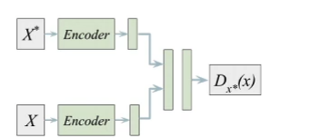
Implicit Density Modeling with Exemplar Models
Fu et al. “EX2: Exploration with Exemplar Models…”
We ned to be able to output densities, but doesn’t necessarily need to produce great samples ⇒ can we explicitly compare the new state to past states?
For each observed state , fit a classifier to classify that state against all past states and use classifier error to obtain density
where is the probability that the classifier assigns as a “positive”
In reality, every state is unique so we regularize the classifier
Heuristic estimation of counts via errors (DNF)
We just need to tell if state is novel or not
Given buffer , fit
So we basically use the error of and actual as a bonus
But what function should we use for ?
-
- as a neural network, but with parameters chosen randomly
We mentioned about how can be seen as Information Gain, it can also be viewed as change in network parameters
So if we forget about IG, there are many other ways to measure this
Stadie et al. 2015:
- encode image observations using auto-encoder
- build predictive model on auto-encoder latent states
- use model error as exploration bonus
Schmidhuber et al. (see, e.g. “Formal Theory of Creativity, Fun, and Intrinsic Motivation):
- exploration bonus for model error
- exploration bonus for model gradient
- many other variations
Suggested Readings
- Schmidhuber. (1992). A Possibility for Implementing Curiosity and Boredom in Model-Building Neural Controllers.
- Stadie, Levine, Abbeel (2015). Incentivizing Exploration in Reinforcement Learning with Deep Predictive Models.
- Osband, Blundell, Pritzel, Van Roy. (2016). Deep Exploration via Bootstrapped DQN.
- Houthooft, Chen, Duan, Schulman, De Turck, Abbeel. (2016). VIME: Variational Information Maximizing Exploration.
- Bellemare, Srinivasan, Ostroviski, Schaul, Saxton, Munos. (2016). Unifying Count-Based Exploration and Intrinsic Motivation.
- Tang, Houthooft, Foote, Stooke, Chen, Duan, Schulman, De Turck, Abbeel. (2016). #Exploration: A Study of Count-Based Exploration for Deep Reinforcement Learning.
- Fu, Co-Reyes, Levine. (2017). EX2: Exploration with Exemplar Models for Deep Reinforcement Learning.
Unsupervised learning of diverse behaviors
What if we want to recover diverse behavior without any reward function at all?
- Learn skills without supervision
- But then use them to accomplish goals
- Learn sub-skills to use with hierarchical reinforcement learning
- Explore the space of possible behaviors
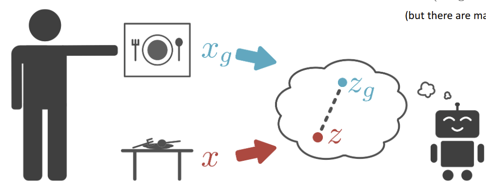
Nair*, Pong*, Bahl, Dalal, Lin, L. Visual Reinforcement Learning with Imagined Goals. ’18 Dalal*, Pong*, Lin*, Nair, Bahl, Levine. Skew-Fit: State-Covering Self-Supervised Reinforcement Learning. ‘19
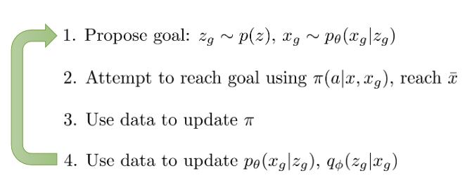
may not be equal to at all…but we will do some updates regardless.
However: This means the model tends to generate states that we’ve already seen (since we sample from ⇒ and we are not exploring very well
We will modify step 4 ⇒ instead of doing MLE: , we will do a weighted MLE:
We want to assign a greater weight to rarely seen actions, and since we’ve used a generator for , we can use
⇒ Note that for any , the entropy increases ⇒ proposing broader and broader goals
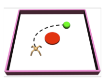
The RL formulation:
- trained to reach goal
- as gets better, the final state gets close to ⇒ becomes more deterministic
To maximize exploration,
This is mainly for gathering data that leads to uniform density over the state distribution ⇒ doesn’t mean the policy is going randomly, what if we want a policy that goes randomly?
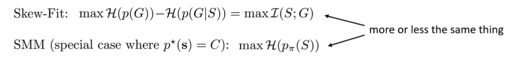
Eysenbach’s Theorem: At test time, an adversary will choose the worst goal G ⇒ Then the best goal distribution use for training would be Hazan, Kakade, Singh, Van Soest. Provably Efficient Maximum Entropy Exploration
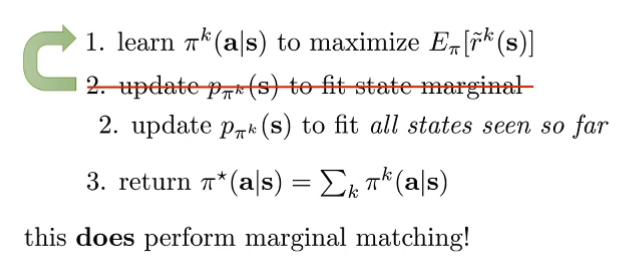
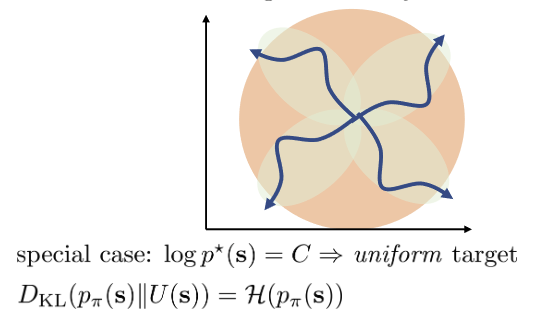
State Marginal Matching (SMM)
Learn to minimize
If we want to use intrinsic motivation, we have:
Note that this reward objective sums to exactly the state-marginal objective above ⇒ However RL is not aware that depends on ⇒ tail chasing problem
We can prove that this is a nash equilibrium for a two-player game
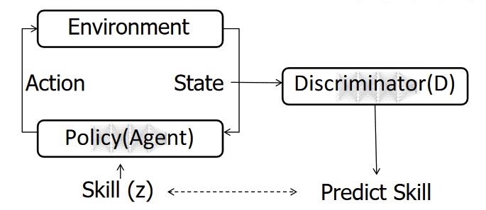
Learning Diverse Skills
- Reaching diverse goals is not the same as performing diverse tasks
- not all behaviors can be captured by goal-reaching
We want reward states for other tasks to be unlikely, one way:
Use a classifier that gives you a softmax output of possibility of s
Connection to mutual information:
Eysenbach, Gupta, Ibarz, Levine. Diversity is All You Need. Gregor et al. Variational Intrinsic Control. 2016