Fundamental Theorem of RL

Fundamental Theorem of RL(Lec 4)

Notations + Markov Property

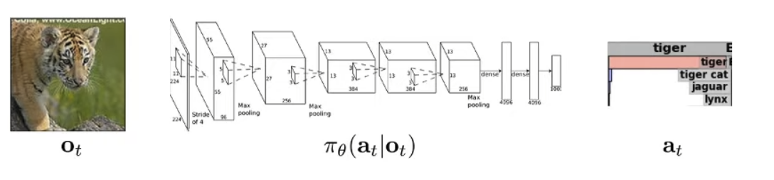
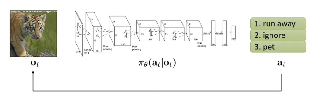
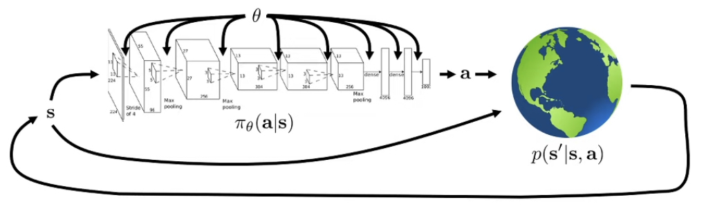
We are actually trying to learn a distribution of action aa given the observation oo, where θ\theta is the parameter of the distribution policy π\pi. we add subscript tt to each term to denote the index in the time-serie since we know in RL that actions are usually correlated.

Sometimes instead of πθ(atot)\pi_\theta (a_t|o_t) we will see πθ(atst)\pi_\theta(a_t|s_t).

ststateπθ(atst)policy (fully observed)otobservationπθ(atot)policys_t \rightarrow \text{state} \\ \pi_\theta(a_t|s_t) \rightarrow \text{policy (fully observed)} \\ o_t \rightarrow \text{observation} \\ \pi_\theta(a_t|o_t) \rightarrow \text{policy}

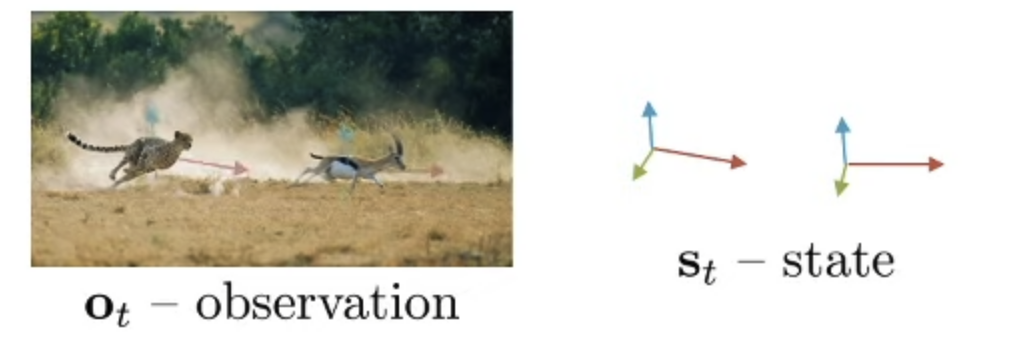
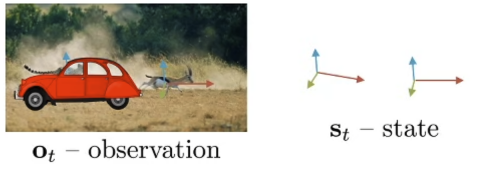
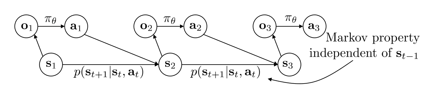
Difference - can use observation to infer state, but sometimes (in this example, car in front of the cheetah) the observation does not give enough information to let us infer state.

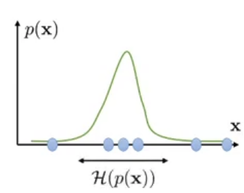
State is the true configuration of the system and observation is something that results from the state which may or may not be enough to deduce the state
🔥
The state is usually assumed to be an Markovian state

Markov property is very important property ⇒ If you want to change the future you just need to focus on current state and your current action

However, is your future state independent of your past observation? In general, observations do not satisfy Markov property

Many RL algorithms in this course requires Markov property

Side note on notation

RL world (Richard Bellman)Robotics (Lev Pontryagin)
sts_t statextx_t state
ata_t actionutu_t action
r(s,a)r(s,a) rewardc(x,u)c(x,u) cost =r(x,u)= -r(x,u)

In general, we want to minimize:

minθEs1:T,a1:T[tc(st,at)]\min_\theta \mathbb{E}_{s_1:T, a_1: T} [\sum_t c(s_t,a_t)]

We can either write the funciton cc as cc or rr, which stands for either (minimize) cost or (maximize) reward

🔥
Notice that we want to maximize the reward (or minimize the cost) under the expectation of the states that we are going to encounter in production / test environment, not training states.

Definition of Markov Chain

M={S,T}M=\{S,T\}
Sstate spacesSstate (discrete or continuous)Ttransition operator described by P(st+1st)S \rightarrow \text{state space} \\ s \in S \rightarrow \text{state (discrete or continuous)} \\ T \rightarrow \text{transition operator described by } \mathbb{P}(s_{t+1}|s_t)

The transition “operator”?

let μt,i=P(st=i),then μt is a vector of probabilities,let Ti,j=P(st+1=isi=j),then μt+1=Tμt\text{let } \mu_{t,i} = \mathbb{P}(s_t = i), \\ \text{then $\vec{\mu}_t$ is a vector of probabilities}, \\ \text{let } T_{i,j} = \mathbb{P}(s_{t+1}=i|s_i=j), \\ \text{then } \vec{\mu}_{t+1} = T\vec{\mu}_t

Definition of Markov Decision Process

M={S,A,T,r}M = \{S,A,T,r\}
Saction space,sSstate (discrete or continuous)Aaction space,aAaction (discrete or continuous)r:S×ARS \rightarrow \text{action space}, \\ s \in S \rightarrow \text{state (discrete or continuous)} \\ A \rightarrow \text{action space}, \\ a \in A \rightarrow \text{action (discrete or continuous)} \\ r: S \times A \rightarrow \mathbb{R} \rightarrow \\
Ttransitional operator (now a tensor)μt,i=P(st=i),ξt,k=P(at=k),So Ti,j,k=P(st+1=ist=j,at=k)μt+1,i=j,kTi,j,kμt,jξt,kT \rightarrow \text{transitional operator (now a tensor)} \\ \mu_{t,i} = \mathbb{P}(s_t=i), \\ \xi_{t,k} = \mathbb{P}(a_t=k), \\ \text{So } T_{i,j,k} = \mathbb{P}(s_{t+1}=i | s_t=j,a_t=k) \\ \mu_{t+1,i} = \sum_{j,k}T_{i,j,k} \mu_{t,j} \xi_{t,k}

Partially Observed Markov Decision Process

M={S,A,O,T,ξ,r}Sstate spacesSstate (discrete or continuous)Aaction spaceaAaction (discrete or continuous)Oobservation spaceoOobservation (discrete or continuous)Ttransition operationξemission probability P(otst)r:S×ARreward functionM = \{S,A,O,T,\xi,r\} \\ S \rightarrow \text{state space} \\ s \in S \rightarrow \text{state (discrete or continuous)} \\ A \rightarrow \text{action space} \\ a \in A \rightarrow \text{action (discrete or continuous)} \\ O \rightarrow \text{observation space} \\ o \in O \rightarrow \text{observation (discrete or continuous)} \\ T \rightarrow \text{transition operation} \\ \xi \rightarrow \text{emission probability $\mathbb{P}(o_t|s_t)$} \\ r: S \times A \rightarrow \mathbb{R} \longrightarrow \text{reward function}

Goal of RL (Finite Horizon / Episodic)

pθ(s1,a1,,sT,aT)undefined
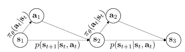
Pθ(τ),where τ represents sequence of trajectory=P(s1)t=1Tπθ(atst)P(st+1st,at)undefinedMarkov chain on (s,a)\underbrace{p_{\theta}(s_1,a_1,\dots,s_T,a_T)}_{\mathclap{\mathbb{P}_\theta(\tau), \text{where $\tau$ represents sequence of trajectory}}}=\mathbb{P}(s_1)\prod_{t=1}^T \underbrace{\pi_{\theta(a_t|s_t)} \mathbb{P}(s_{t+1}|s_t,a_t)}_{\mathclap{\text{Markov chain on $(s,a)$}}}

So our goal is to maximize the expectation of rewards

θ=arg maxθEτpθ[tr(st,at)]\theta^* = \argmax_\theta \mathbb{E}_{\tau \sim p_\theta}[\sum_t r(s_t,a_t)]
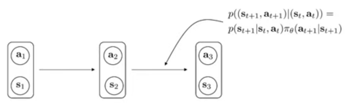
Group action and state together to form augmented states
Augmented states form a Markov Chain.

The markov chain can be described using:

[st+1at+1]=T[stat][st+kat+k]=Tk[stat]\begin{split} \begin{bmatrix} s_{t+1} \\ a_{t+1} \end{bmatrix} = T\begin{bmatrix} s_t \\ a_t \end{bmatrix} \\ \begin{bmatrix} s_{t+k} \\ a_{t+k} \end{bmatrix} = T^k \begin{bmatrix} s_t \\ a_t \end{bmatrix} \end{split}

So now we can modify the goal a bit towards the markov chain.

θ=arg maxθEτpθ(τ)[tr(st,at)]=arg maxθt=1TE(st,at)pθ(st,at)[r(st,at)]\begin{split} \theta^* &= \argmax_\theta \mathbb{E}_{\tau \sim p_\theta(\tau)}[\sum_t r(s_t,a_t)] \\ &= \argmax_\theta \sum_{t=1}^T \mathbb{E}_{(s_t,a_t)\sim p_\theta(s_t,a_t)}[r(s_t,a_t)] \end{split}

Goal of RL (Infinite Horizon)

What if T=T = \infin? (Infinite horizon)

  1. We need some way to make objective finite
    1. Use average award θ=arg maxθ1TEτpθ(τ)[tr(st,at)]\theta^* = \argmax_\theta \frac{1}{T}\mathbb{E}{\tau \sim p\theta(\tau)}[\sum_t r(s_t,a_t)]
    1. Use discounts

Q: Does p(st,at)p(s_t,a_t) converge to a stationary distribution as tt \rightarrow \infin?

Ergodic Property: Every state can transition into another state with a non-zero probability.

“Stationary”: The same before and after transition

μ=Tμundefinedstationary means the state is same and before after transition\underbrace{\mu = T \mu}_{\text{stationary means the state is same and before after transition}}
(TI)μ=0(T-I)\mu = 0

This means that μ\mu is an eigenvector of TT with eigenvalue of 1 (always exists under some regularity conditions)

μ=pθ(s,a)stationary distribution\mu = p_\theta(s,a) \rightarrow \text{stationary distribution}

As tt goes further and further from infinity, the reward terms starts to get dominated by the stationary distribution (we have almost inifite μ\mu states and a finite non-stationary action/state pairs

limTθ=limTarg maxθ1Tt=1TE(st,at)pθ(st,at)[r(st,at)]=arg maxθE(s,a)pθ(s,a)[r(s,a)]\begin{split} \lim_{T \rightarrow \infin} \theta^* &= \lim_{T \rightarrow \infin} \argmax_\theta \frac{1}{T}\sum_{t=1}^T \mathbb{E}_{(s_t,a_t) \sim p\theta(s_t,a_t)}[r(s_t,a_t)] \\ &= \argmax_{\theta} \mathbb{E}_{(s,a) \sim p_\theta(s,a)}[r(s,a)] \end{split}

Expectations and Stochastic Systems

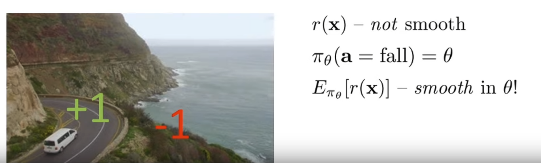
RL is about maximizing the expectation of rewards. And expectations can be continuous in the parameters of the corresponding distributions even when the function we are taking expectation of is itself highly discontinuous. Because of this property we can use smooth optimization methods like Gradient Descent
📌
Because the distribution of the probability of getting a reward usually has a continuous PDF.

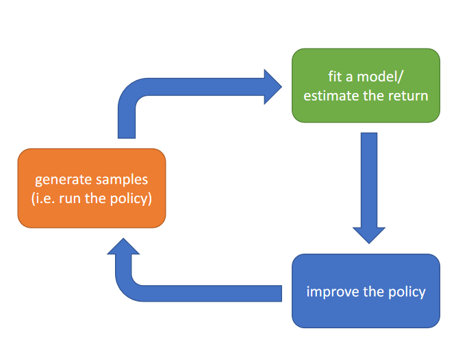
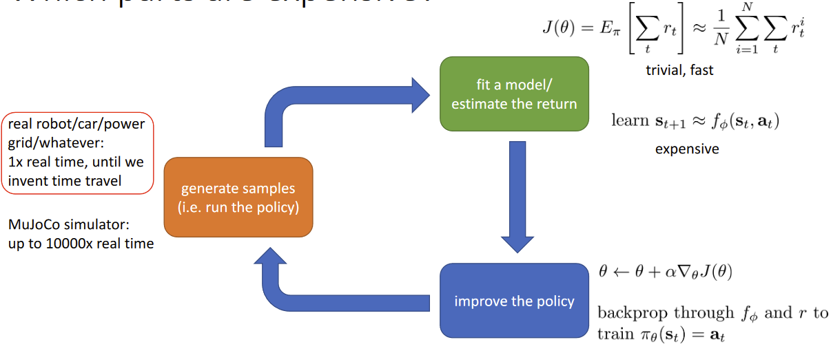
High-level anatomy of reinforcement learning algorithms

Which parts are expensive?

Value Function & Q Function

Remember that RL problems are framed as argmax of expectation of rewards, but how do we actually deal with the expectations?

📌
Write it out recursively!

We can write this expectation out explicitly as a nested expectation (looks like a DP algorithm!)

Eτp(s1)[t=1Tr(st,at)]=Es1p(s1)[Ea1π(a1s1)[r(s1,a1)+Es2p(s2s1,a1)[Ea2π(a2s2)[r(s2,a2)+s2]s1,a1]s1]]\mathbb{E}_{\tau \sim p(s_1)}[\sum_{t=1}^T r(s_t,a_t)] = \\ \mathbb{E}_{s_1 \sim p(s_1)}[\mathbb{E}_{a_1 \sim \pi(a_1|s_1)}[r(s_1,a_1)+\mathbb{E}_{s_2 \sim p(s_2|s_1,a_1)}[\mathbb{E}_{a_2 \sim \pi(a_2|s_2)}[r(s_2,a_2)+\cdots|s_2]|s_1,a_1]|s_1]]
Looks like its messy, but what if we have a function that tells us what value inside the Ea1π(a1s1)\mathbb{E}_{a_1 \sim \pi(a_1|s_1)} is? Specifically, its the value of r(s1,a1)+Es2p(s2s1,a1)[Ea2π(a2s2)[r(s2,a2)+s2]s1,a1]r(s_1,a_1)+\mathbb{E}_{s_2 \sim p(s_2|s_1,a_1)}[\mathbb{E}{a_2 \sim \pi(a_2|s_2)}[r(s_2,a_2)+\cdots|s_2]|s_1,a_1] We will define it as our QQ function
Q(s1,a1)=r(s1,a1)+Es2p(s2s1,a1)[Ea2π(a2s2)[r(s2,a2)+s2]s1,a1]Q(s_1,a_1) = r(s_1,a_1)+\mathbb{E}_{s_2 \sim p(s_2|s_1,a_1)}[\mathbb{E}_{a_2 \sim \pi(a_2|s_2)}[r(s_2,a_2)+\cdots|s_2]|s_1,a_1]

Then our equation is simplified into

Eτp(s1)[t=1Tr(st,at)]=Es1p(s1)[Ea1π(a1s1)[Q(s1,a1)s1]]\mathbb{E}_{\tau \sim p(s_1)}[\sum_{t=1}^T r(s_t,a_t)] = \\ \mathbb{E}_{s_1 \sim p(s_1)}[\mathbb{E}_{a_1 \sim \pi(a_1|s_1)}[Q(s_1,a_1)|s_1]]

It’s a lot easier to modify the parameter θ\theta of πθ(a1s1)\pi_\theta(a_1|s_1) if Q(s1,a1)Q(s_1,a_1) is known


Q-Function Definition

Qπ(st,at)=t=tTEπθ[r(st,at)st,at]total reward from taking at in stQ^{\pi}(s_t,a_t)=\sum_{t'=t}^T \mathbb{E}_{\pi_\theta}[r(s_{t'},a_{t'})|s_t,a_t] \rightarrow \text{total reward from taking $a_t$ in $s_t$}

Value Function Definition

Vπ(st)=t=tTEπθ[r(st,at)st]total reward from stV^{\pi}(s_t)=\sum_{t'=t}^T \mathbb{E}_{\pi_\theta}[r(s_{t'},a_{t'})|s_t] \rightarrow \text{total reward from $s_t$}
Vπ(st)=Eatπ(atst)[Qπ(st,at)]V^{\pi}(s_t) = \mathbb{E}_{a_t \sim \pi(a_t|s_t)}[Q^{\pi}(s_t,a_t)]

Now Es1p(s1)[Vπ(s1)]\mathbb{E}_{s_1}\sim p(s_1)[V^{\pi}(s_1)] is the RL objective.

To use those two functions:

If we have policy π\pi, and we know Qπ(s,a)Q^{\pi}(s,a), then we can improve π\pi:

set π(as)=1 if a=arg maxaQπ(s,a)\text{set } \pi^{'}(a|s)=1 \text{ if } a = \argmax_a Q^{\pi}(s,a)

(This policy is at least as good as π\pi and probably better)

OR

Compute gradient to increase the probability of good actions aa if Qπ(s,a)>Vπ(s)Q^{\pi}(s,a) > V^{\pi}(s), then aa is better than average. Recall that Vπ(s)=E[Qπ(s,a)]V^{\pi}(s) = \mathbb{E}[Q^{\pi}(s,a)] under π(as)\pi(a|s).

Modify π(as)\pi(a|s) to increase the probability of a if Qπ(s,a)>Vπ(s)Q^{\pi}(s,a) > V^{\pi}(s)

Bellman Operator

First defined in fixed Q-Iteration

Information Theory (LEC 14)

Some useful identities:

  1. p(x)p(x) - distribution (over observations x)
  1. H(p(x))=Exp(x)[logp(x)]H(p(x))= -\mathbb{E}_{x \sim p(x)}[\log p(x)] ⇒ entropy (how “broad” p(x) is)
  1. I(x;y)=DKL(p(x,y)p(x)p(y))=E(x,y)p(x,y)[logp(x,y)p(x)p(y)]=H(p(y))H(p(yx))I(x;y) = D_{KL}(p(x,y)||p(x)p(y)) = \mathbb{E}_{(x,y) \sim p(x,y)}[\log \frac{p(x,y)}{p(x) p(y)}] = H(p(y)) - H(p(y|x))
    1. mutual information between two variables
    1. reduction in entropy after knowing xx
    1. See “empowerment” (Polani et al.) for a typical use
      1. I(st+1;at)=H(st+1)H(st+1at)I(s_{t+1}; a_t) = H(s_{t+1}) - H(s_{t+1}|a_t)
      1. Can be viewed as quantifying “control authority” in an information-theoretic way