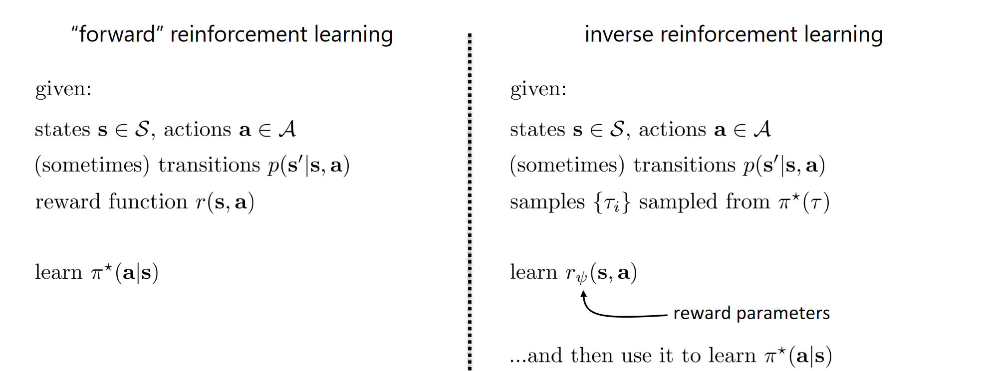
So far, we’ve hand designed reward function to define a task What if we want to learn the reward function from observing an expert and then apply reinforcement learning through the learned reward function? Apply approximate optimality model(Control as an Inference model) from last time, but now learn the reward 📢
Inverse Reinforcement Learning : Infer reward functions from demonstrations
Standard Imitation Learning
Copy the actions performed by the expert No reasoning about outcomes of actions Human Imitation Learning
Copy the intent of the expert might take very different actions!
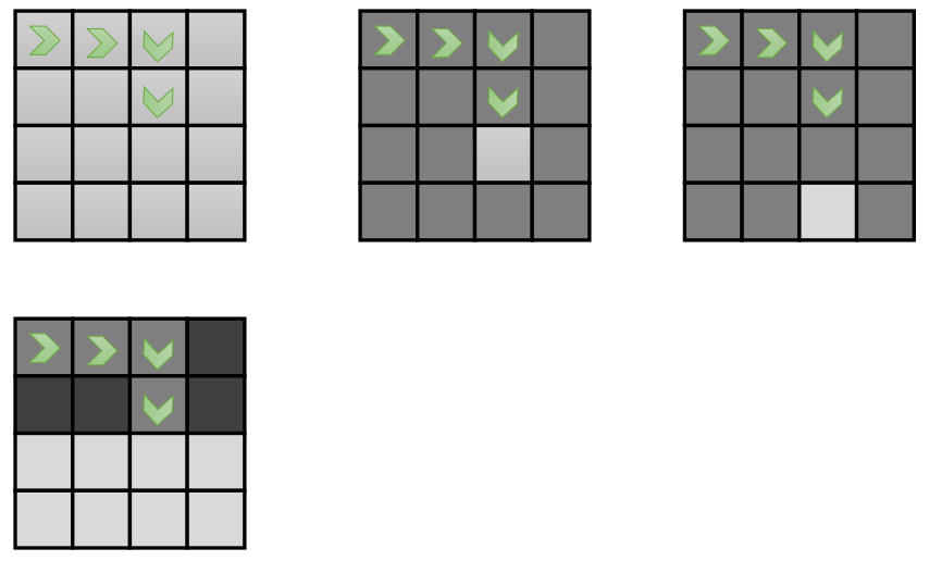
Problem: many reward functions can explain the same behavior
Top-left: behavior, top-center: possible reward block, top-right: possible reward block, bottom-left: possoble reward blocks Reward Parameterization
Traditional Linear Formulationr ψ ( s , a ) = ∑ i ψ i f i ( s , a ) = ψ ⊤ f ( s , a ) r_\psi(s,a) = \sum_i \psi_i f_i(s,a) = \psi^{\top} f(s,a) r ψ ( s , a ) = ∑ i ψ i f i ( s , a ) = ψ ⊤ f ( s , a ) f ( s , a ) f(s,a) f ( s , a ) Neural Net Formulationr ψ ( s , a ) r_\psi(s,a) r ψ ( s , a )
Feature Matching IRL Linear Reward Function
r ψ ( s , a ) = ∑ i ψ i f i ( s , a ) = ψ ⊤ f ( s , a ) r_\psi(s,a) = \sum_i \psi_i f_i(s,a) = \psi^{\top} f(s,a) r ψ ( s , a ) = i ∑ ψ i f i ( s , a ) = ψ ⊤ f ( s , a ) If features f f f
Let π r ψ \pi^{r_\psi} π r ψ r ψ r_\psi r ψ
If we pick ψ \psi ψ E π r ψ [ f ( s , a ) ] = E π ∗ [ f ( s , a ) ] \mathbb{E}_{\pi^{r_\psi}}[f(s,a)] = \mathbb{E}_{\pi^*}[f(s,a)] E π r ψ [ f ( s , a )] = E π ∗ [ f ( s , a )]
We can estimate the optimal policy expectation by averaging expert samples But Multiple different ψ \psi ψ So now if we choose to use max margin principle (similar to SVM):
max ψ , m m s.t. ψ ⊤ E π ∗ [ f ( s , a ) ] ≥ max π ∈ Π ψ ⊤ E π [ f ( s , a ) ] + m \max_{\psi, m} m \\
\text{s.t.} \\
\psi^{\top} \mathbb{E}_{\pi^*}[f(s,a)] \ge \max_{\pi \in \Pi} \psi^{\top} \mathbb{E}_\pi [f(s,a)] + m ψ , m max m s.t. ψ ⊤ E π ∗ [ f ( s , a )] ≥ π ∈ Π max ψ ⊤ E π [ f ( s , a )] + m It’s a heuristic ⇒ not necessarily mean we’ll recover the true weight of expert’s reward function, but it’s a reasonable heuristic. But we need to somehow weight the margin by similarity between π ∗ \pi^* π ∗ π \pi π apply the “SVM trick”, the problem becomes
min ψ 1 2 ∣ ∣ ψ ∣ ∣ 2 s.t. ψ ⊤ E π ∗ [ f ( s , a ) ] ≥ max π ∈ Π ψ ⊤ E π [ f ( s , a ) ] + 1 \min_\psi \frac{1}{2} ||\psi||^2 \\
\text{s.t.} \\
\psi^{\top} \mathbb{E}_{\pi^*}[f(s,a)] \ge \max_{\pi \in \Pi} \psi^\top \mathbb{E}_{\pi}[f(s,a)] + 1 ψ min 2 1 ∣∣ ψ ∣ ∣ 2 s.t. ψ ⊤ E π ∗ [ f ( s , a )] ≥ π ∈ Π max ψ ⊤ E π [ f ( s , a )] + 1 Let’s also add in a measure of difference in policy
min ψ 1 2 ∣ ∣ ψ ∣ ∣ 2 s.t. ψ ⊤ E π ∗ [ f ( s , a ) ] ≥ max π ∈ Π ψ ⊤ E π [ f ( s , a ) ] + D ( π , π ∗ ) \min_\psi \frac{1}{2} ||\psi||^2 \\
\text{s.t.} \\
\psi^{\top} \mathbb{E}_{\pi^*}[f(s,a)] \ge \max_{\pi \in \Pi} \psi^\top \mathbb{E}_{\pi}[f(s,a)] + D(\pi, \pi^*) ψ min 2 1 ∣∣ ψ ∣ ∣ 2 s.t. ψ ⊤ E π ∗ [ f ( s , a )] ≥ π ∈ Π max ψ ⊤ E π [ f ( s , a )] + D ( π , π ∗ ) Note:
D ( ⋅ ) D(\cdot) D ( ⋅ )
Issues:
Maximizing the margin is a bit arbitrary“Find a reward function which the expert’s policy is clearly better than any other policies” No clear model of expert sub-optimalityCan add slack variables just like in SVM to allow sub-optimality Messy constrained optimization problemNot good for deep learning
Abbeel & Ng: Apprenticeship learning via inverse reinforcement learning
Ratliff et al: Maximum margin planning
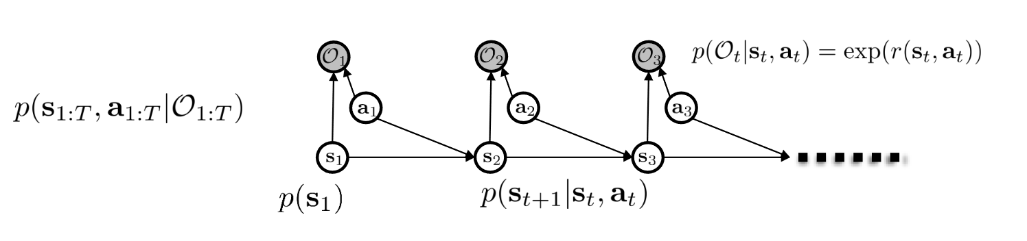
Optimal Control as a Model of Human Behavior p ( s 1 : T , a 1 : T ) = ? p(s_{1:T}, a_{1:T}) = ? p ( s 1 : T , a 1 : T ) = ? What we know:
p ( O t ∣ s t , a t ) = exp ( r ( s t , a t ) ) p(O_t|s_t,a_t) = \exp(r(s_t,a_t)) p ( O t ∣ s t , a t ) = exp ( r ( s t , a t )) But we can do optimality inference (What is the probability of trajectory given optimality)
p ( τ ∣ O 1 : T ) = p ( τ , O 1 : T ) p ( O 1 : T ) ∝ p ( τ ) ∏ t exp ( r ( s t , a t ) ) = p ( τ ) exp ( ∑ t r ( s t , a t ) ) \begin{split}
p(\tau|O_{1:T}) &= \frac{p(\tau, O_{1:T})}{p(O_{1:T})} \\
&\propto p(\tau) \prod_t \exp(r(s_t,a_t)) \\
&\quad = p(\tau) \exp(\sum_{t} r(s_t,a_t))
\end{split} p ( τ ∣ O 1 : T ) = p ( O 1 : T ) p ( τ , O 1 : T ) ∝ p ( τ ) t ∏ exp ( r ( s t , a t )) = p ( τ ) exp ( t ∑ r ( s t , a t )) Learning the optimality variable p ( O t ∣ s t , a t , ψ ) = exp ( r ψ ( s t , a t ) ) p(O_t|s_t,a_t,\psi) = \exp(r_\psi(s_t,a_t)) p ( O t ∣ s t , a t , ψ ) = exp ( r ψ ( s t , a t )) p ( τ ∣ O 1 : T , ψ ) ∝ p ( τ ) undefined turns out we can ignore because independent of ψ exp ( ∑ t r ψ ( s t , a t ) ) p(\tau|O_{1:T}, \psi) \propto \underbrace{p(\tau)}_{\mathclap{\text{turns out we can ignore because independent of $\psi$}}} \exp(\sum_t r_\psi(s_t,a_t)) p ( τ ∣ O 1 : T , ψ ) ∝ turns out we can ignore because independent of ψ p ( τ ) exp ( t ∑ r ψ ( s t , a t )) Maximum Likelihood Learning:
max ψ 1 N ∑ i = 1 N log p ( τ i ∣ O 1 : T , ψ ) = max ψ 1 N ∑ i = 1 N r ψ ( τ i ) − log Z \begin{split}
\max_{\psi} \frac{1}{N} \sum_{i=1}^N \log p(\tau_i | O_{1:T}, \psi)
&= \max_{\psi} \frac{1}{N} \sum_{i=1}^N r_\psi(\tau_i) - \log Z
\end{split}
ψ max N 1 i = 1 ∑ N log p ( τ i ∣ O 1 : T , ψ ) = ψ max N 1 i = 1 ∑ N r ψ ( τ i ) − log Z 📢
Why we add a negative
log Z \log Z log Z term here? Because if we only want to max rewards, we can make them high everywhere and the learned reward function is basically unusable.
Z Z Z is called the
partition function IRL Parition Function Z = ∫ p ( τ ) exp ( r ψ ( τ ) ) d τ Z = \int p(\tau) \exp(r_\psi(\tau)) d\tau Z = ∫ p ( τ ) exp ( r ψ ( τ )) d τ 🤧
Wow! That looks like an integral over all possible trajectories and we know that this is probably intractable, but let’s plug this into maximum likelihood learning and see what happens anyway!
∇ ψ L = 1 N ∑ i = 1 N ∇ ψ r ψ ( τ i ) − 1 Z ∫ p ( τ ) exp ( r ψ ( τ ) ) ∇ ψ r ψ ( τ ) d τ = E τ ∼ π ∗ ( τ ) [ ∇ ψ r ψ ( τ i ) ] − E τ ∼ p ( τ ∣ O 1 : T , ψ ) [ ∇ ψ r ψ ( τ ) ] \begin{split}
\nabla_\psi L
&= \frac{1}{N} \sum_{i=1}^N \nabla_\psi r_\psi(\tau_i) - \frac{1}{Z} \int p(\tau) \exp(r_\psi(\tau)) \nabla_\psi r_\psi(\tau) d\tau \\
&= \mathbb{E}_{\tau \sim \pi^*(\tau)}[\nabla_\psi r_\psi(\tau_i)] - \mathbb{E}_{\tau \sim p(\tau|O_{1:T},\psi)}[\nabla_{\psi} r_\psi(\tau)]
\end{split} ∇ ψ L = N 1 i = 1 ∑ N ∇ ψ r ψ ( τ i ) − Z 1 ∫ p ( τ ) exp ( r ψ ( τ )) ∇ ψ r ψ ( τ ) d τ = E τ ∼ π ∗ ( τ ) [ ∇ ψ r ψ ( τ i )] − E τ ∼ p ( τ ∣ O 1 : T , ψ ) [ ∇ ψ r ψ ( τ )] OK, this looks reasonableIncrease rewards at data points that we saw in the expert data Decrease rewards at data points in the soft optimal policy of our current reward estimate Let’s proceed and estimate this expectation E τ ∼ p ( τ ∣ O 1 : T , ψ ) [ ∇ ψ r ψ ( τ ) ] = E τ ∼ p ( τ ∣ O 1 : T , ψ ) [ ∇ ψ ∑ t = 1 T r ψ ( s t , a t ) ] = ∑ t = 1 T E ( s t , a t ) ∼ p ( s t , a t ∣ O 1 : T , ψ ) [ ∇ ψ r ψ ( s t , a t ) ] \begin{split}
\mathbb{E}_{\tau\sim p(\tau|O_{1:T},\psi)} [\nabla_\psi r_\psi (\tau)]
&= \mathbb{E}_{\tau\sim p(\tau|O_{1:T},\psi)} [\nabla_\psi \sum_{t=1}^T r_\psi(s_t,a_t)] \\
&= \sum_{t=1}^T \mathbb{E}_{(s_t,a_t) \sim p(s_t,a_t|O_{1:T},\psi)}[\nabla_\psi r_\psi(s_t,a_t)]
\end{split} E τ ∼ p ( τ ∣ O 1 : T , ψ ) [ ∇ ψ r ψ ( τ )] = E τ ∼ p ( τ ∣ O 1 : T , ψ ) [ ∇ ψ t = 1 ∑ T r ψ ( s t , a t )] = t = 1 ∑ T E ( s t , a t ) ∼ p ( s t , a t ∣ O 1 : T , ψ ) [ ∇ ψ r ψ ( s t , a t )] Note:
p ( s t , a t ) ∣ O 1 : T , ψ ) = p ( a t ∣ s t , O 1 : T , ψ ) undefined = β ( s t , a t ) β ( s t ) p ( s t ∣ O 1 : T , ψ ) undefined ∝ α ( s t ) β ( s t ) ∝ β ( s t , a t ) α ( s t ) \begin{split}
p(s_t,a_t)|O_{1:T}, \psi)
&= \overbrace{p(a_t|s_t, O_{1:T}, \psi)}^{\mathclap{=\frac{\beta(s_t,a_t)}{\beta(s_t)}}} \underbrace{p(s_t|O_{1:T},\psi)}_{\mathclap{\propto \alpha (s_t) \beta(s_t)}} \\
&\propto \beta(s_t,a_t) \alpha(s_t)
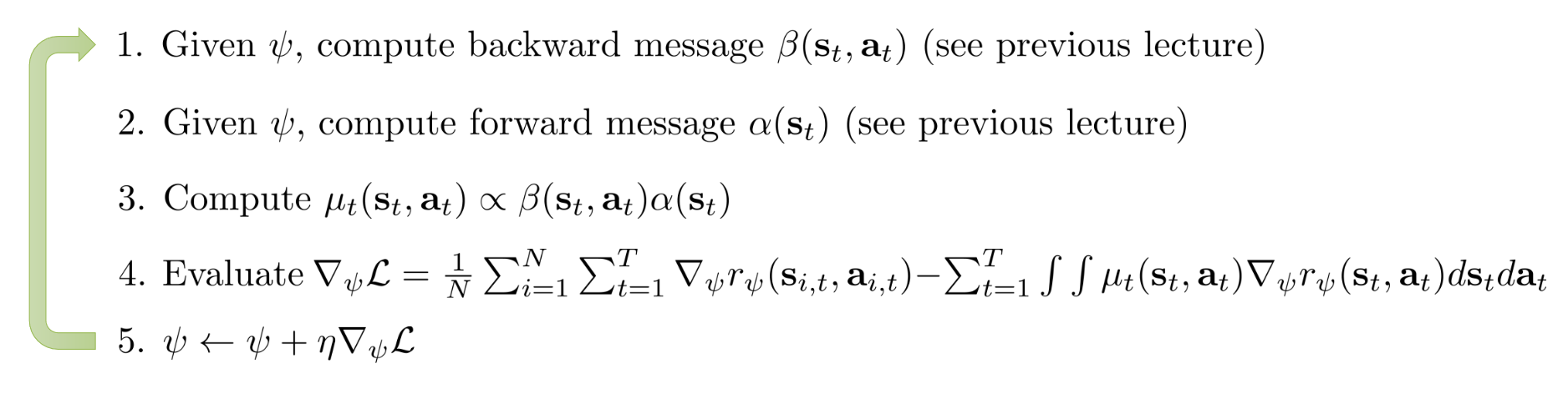
\end{split} p ( s t , a t ) ∣ O 1 : T , ψ ) = p ( a t ∣ s t , O 1 : T , ψ ) = β ( s t ) β ( s t , a t ) ∝ α ( s t ) β ( s t ) p ( s t ∣ O 1 : T , ψ ) ∝ β ( s t , a t ) α ( s t ) Let μ t ( s t , a t ) ∝ β ( s t , a t ) α ( s t ) \mu_t(s_t,a_t) \propto \beta(s_t,a_t) \alpha(s_t) μ t ( s t , a t ) ∝ β ( s t , a t ) α ( s t )
E τ ∼ p ( τ ∣ O 1 : T , ψ ) [ ∇ ψ r ψ ( τ ) ] = ∑ t = 1 T E ( s t , a t ) ∼ p ( s t , a t ∣ O 1 : T , ψ ) [ ∇ ψ r ψ ( s t , a t ) ] = ∑ t = 1 T ∫ ∫ μ t ( s t , a t ) ∇ ψ r ψ ( s t , a t ) d s t d a t = ∑ t = 1 T μ ⃗ ⊤ ∇ ψ r ⃗ ψ \begin{split}
\mathbb{E}_{\tau\sim p(\tau|O_{1:T},\psi)} [\nabla_\psi r_\psi (\tau)]
&= \sum_{t=1}^T \mathbb{E}_{(s_t,a_t) \sim p(s_t,a_t|O_{1:T},\psi)}[\nabla_\psi r_\psi(s_t,a_t)] \\
&=\sum_{t=1}^T \int \int \mu_t(s_t,a_t) \nabla_\psi r_\psi(s_t,a_t) ds_t da_t \\
&=\sum_{t=1}^T \vec{\mu}^\top \nabla_\psi \vec{r}_\psi
\end{split} E τ ∼ p ( τ ∣ O 1 : T , ψ ) [ ∇ ψ r ψ ( τ )] = t = 1 ∑ T E ( s t , a t ) ∼ p ( s t , a t ∣ O 1 : T , ψ ) [ ∇ ψ r ψ ( s t , a t )] = t = 1 ∑ T ∫∫ μ t ( s t , a t ) ∇ ψ r ψ ( s t , a t ) d s t d a t = t = 1 ∑ T μ ⊤ ∇ ψ r ψ Note: This works for small and discrete state and action spaces so we can estimate μ ⃗ \vec{\mu} μ
MaxEnt IRL Ziebart et al. 2008: Maximum Entropy Inverse Reinforcement Learning Its nice because
If r ψ ( s t , a t ) = ψ ⊤ f ( s t , a t ) r_\psi(s_t,a_t) = \psi^{\top} f(s_t,a_t) r ψ ( s t , a t ) = ψ ⊤ f ( s t , a t ) max ψ H ( π r ψ ) \max_{\psi} H(\pi^{r_\psi}) max ψ H ( π r ψ ) E π r ψ [ f ] = E π ∗ [ f ] \mathbb{E}_{\pi^{r_\psi}}[f] = \mathbb{E}_{\pi^*}[f] E π r ψ [ f ] = E π ∗ [ f ]
Extending to high dimensional spaces MaxEnt IRL so far requiresSolving for (soft) optial policy in the inner loop Enumerting all state-action tuples for visitation frequency and gradient To apply this in practical problem settings, we need to handleLarge and continuous state and action spaces States obtained via sampling only Unknown dynamicscausing the naive method of computing backward/forward messages unstable
Assume we can sample from the real environment
Idea:
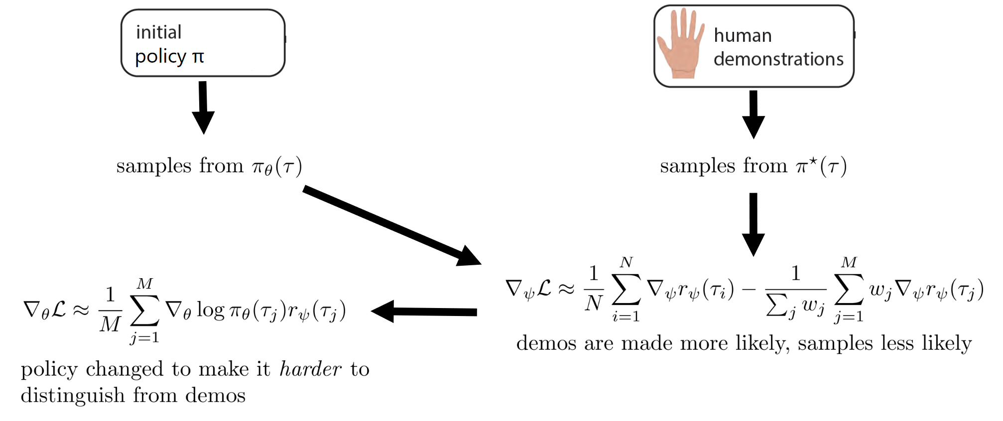
Learn p ( a t ∣ s t , O 1 : T , ψ ) p(a_t|s_t, O_{1:T}, \psi) p ( a t ∣ s t , O 1 : T , ψ ) { τ j } \{ \tau_j \} { τ j } ∇ ψ L ≈ 1 N ∑ i = 1 N ∇ ψ r ψ ( τ i ) − 1 M ∑ j = 1 M ∇ ψ r ψ ( τ j ) \nabla_{\psi} L \approx \frac{1}{N} \sum_{i=1}^N \nabla_\psi r_\psi(\tau_i) - \frac{1}{M} \sum_{j=1}^M \nabla_\psi r_\psi(\tau_j) ∇ ψ L ≈ N 1 ∑ i = 1 N ∇ ψ r ψ ( τ i ) − M 1 ∑ j = 1 M ∇ ψ r ψ ( τ j ) Looks expensive, what if we use “lazy” policy optimization ⇒ instead of learning a policy every time can we optimize a bit? Improve p ( a t ∣ s t , O 1 : T , ψ ) p(a_t|s_t, O_{1:T}, \psi) p ( a t ∣ s t , O 1 : T , ψ ) But now the estimator is now biased; wrong distributionUse importance sampling∇ ψ L ≈ 1 N ∑ i = 1 N ∇ ψ r ψ ( τ i ) − 1 ∑ j w j ∑ j = 1 M w j ∇ ψ r ψ ( τ j ) \nabla_{\psi} L \approx \frac{1}{N} \sum_{i=1}^N \nabla_\psi r_\psi(\tau_i) - \frac{1}{\sum_j w_j} \sum_{j=1}^M w_j \nabla_\psi r_\psi(\tau_j) ∇ ψ L ≈ N 1 ∑ i = 1 N ∇ ψ r ψ ( τ i ) − ∑ j w j 1 ∑ j = 1 M w j ∇ ψ r ψ ( τ j )
Importance weights
w j = p ( τ ) exp ( r ψ ( τ j ) ) π ( τ j ) = p ( s 1 ) ∏ t p ( s t + 1 ∣ s t , a t ) exp ( r ψ ( s t , a t ) ) p ( s 1 ) ∏ t p ( s t + 1 ∣ s t , a t ) π ( a t ∣ s t ) = exp ( ∑ t r ψ ( s t , a t ) ) ∏ t π ( a t ∣ s t ) \begin{split}
w_j
&= \frac{p(\tau) \exp(r_\psi(\tau_j))}{\pi(\tau_j)} \\
& = \frac{p(s_1)\prod_t p(s_{t+1}|s_t,a_t) \exp(r_\psi(s_t,a_t))}{p(s_1) \prod_t p(s_{t+1}|s_t,a_t) \pi(a_t|s_t)} \\
&=\frac{\exp(\sum_t r_\psi(s_t,a_t))}{\prod_t \pi(a_t|s_t)}
\end{split} w j = π ( τ j ) p ( τ ) exp ( r ψ ( τ j )) = p ( s 1 ) ∏ t p ( s t + 1 ∣ s t , a t ) π ( a t ∣ s t ) p ( s 1 ) ∏ t p ( s t + 1 ∣ s t , a t ) exp ( r ψ ( s t , a t )) = ∏ t π ( a t ∣ s t ) exp ( ∑ t r ψ ( s t , a t )) Each policy update with respect to r ψ r_\psi r ψ
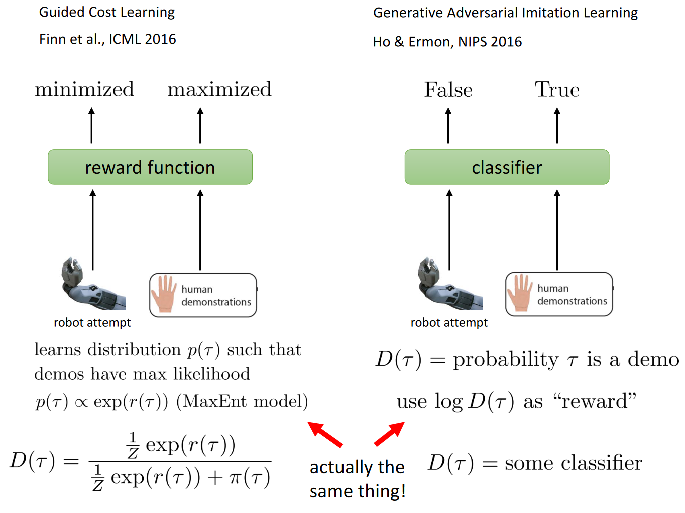
IRL and GANs The IRL algorithm described earlier looks like a game “Policy trying to look as good as the expert, reward trying to differentiate experts from policy”
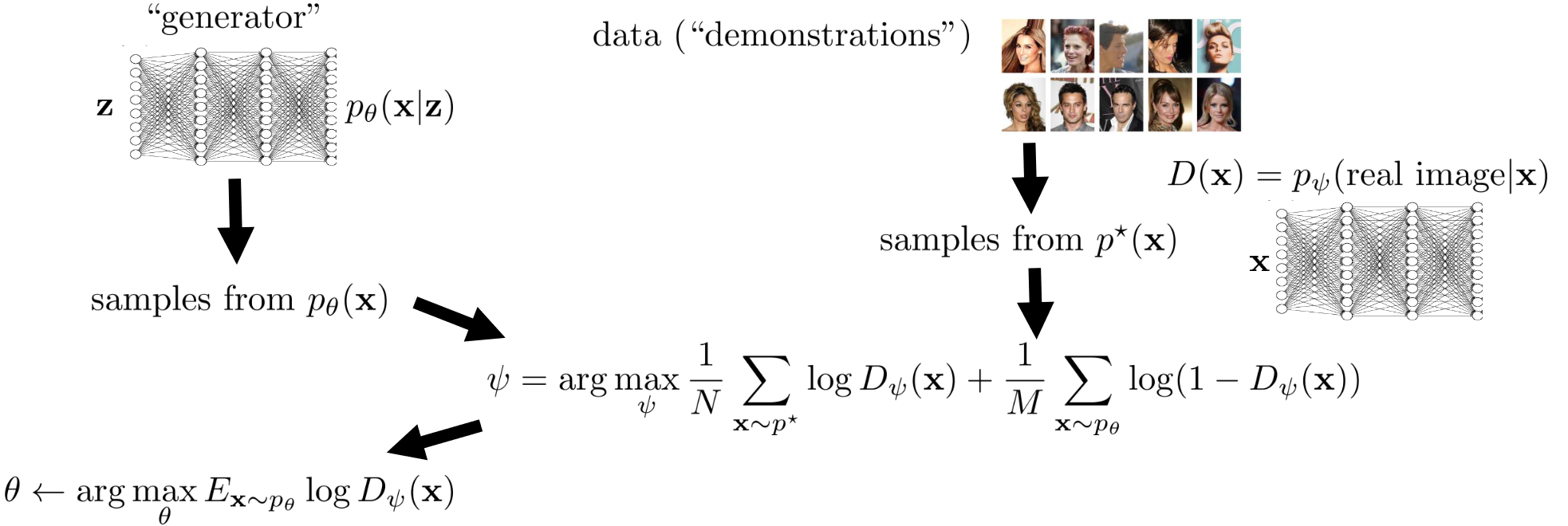
Generative Adversarial Networks (GANs) Inverse RL as a GAN Finn*, Christiano* et al. “A Connection Between Generative Adversarial Networks, Inverse Reinforcement Learning, and Energy-Based Models.” In GAN, the optimal discriminator is
D ∗ ( x ) = p ∗ ( x ) p θ ( x ) + p ∗ ( x ) D^*(x) = \frac{p^*(x)}{p_\theta(x) + p^*(x)} D ∗ ( x ) = p θ ( x ) + p ∗ ( x ) p ∗ ( x ) The density distribution of real and fake if the discriminator is converged We know for IRL, the optimal policy approaches
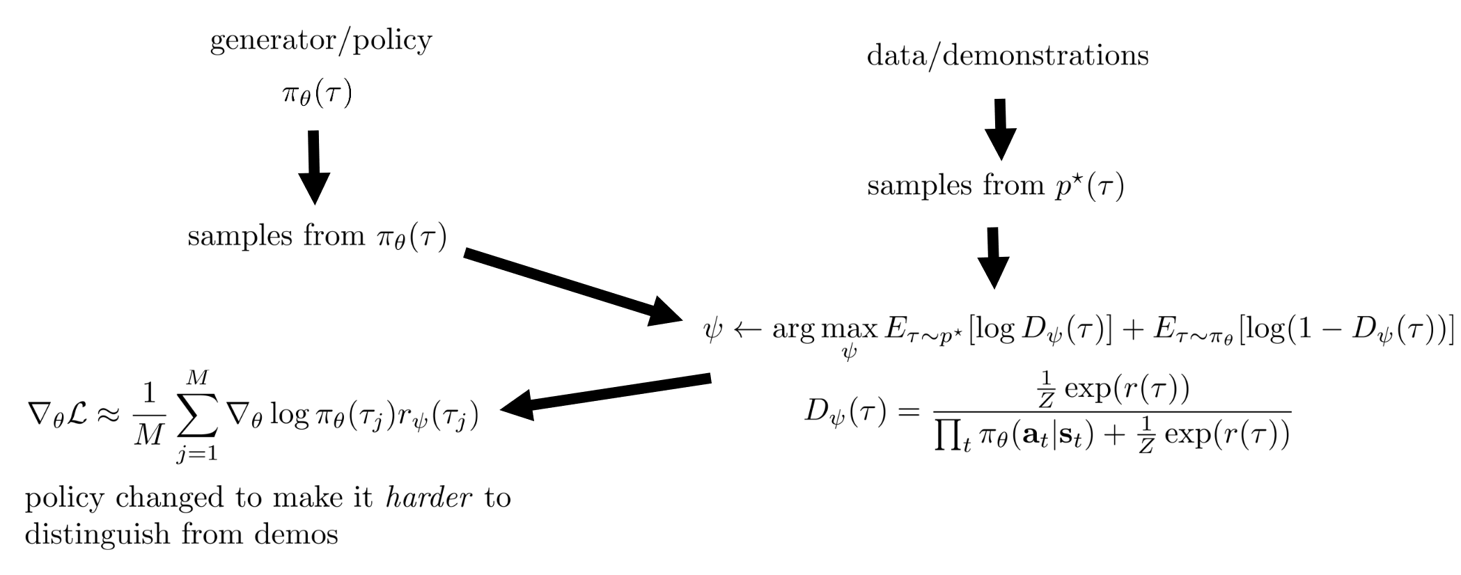
π θ ( τ ) ∝ p ( τ ) exp ( r ψ ( τ ) ) \pi_\theta(\tau) \propto p(\tau) \exp(r_\psi(\tau)) π θ ( τ ) ∝ p ( τ ) exp ( r ψ ( τ )) The parameterization for discriminator for IRL is:
D ψ ( τ ) = p ( τ ) 1 Z exp ( r ( τ ) ) p θ ( τ ) + p ( τ ) 1 Z exp ( r ( τ ) ) = p ( τ ) Z − 1 exp ( r ( τ ) ) p ( τ ) ∏ t π θ ( a t ∣ s t ) + p ( τ ) Z − 1 exp ( r ( τ ) ) = Z − 1 exp ( r ( τ ) ) ∏ t π θ ( a t ∣ s t ) + Z − 1 exp ( r ( τ ) ) \begin{split}
D_\psi(\tau)
&= \frac{p(\tau) \frac{1}{Z} \exp(r(\tau))}{p_\theta(\tau) + p(\tau) \frac{1}{Z}\exp(r(\tau))} \\
&= \frac{p(\tau) Z^{-1} \exp(r(\tau))}{p(\tau)\prod_t \pi_\theta(a_t|s_t) + p(\tau) Z^{-1} \exp(r(\tau))} \\
&= \frac{Z^{-1} \exp(r(\tau))}{\prod_t \pi_\theta(a_t|s_t) + Z^{-1}\exp(r(\tau))}
\end{split} D ψ ( τ ) = p θ ( τ ) + p ( τ ) Z 1 exp ( r ( τ )) p ( τ ) Z 1 exp ( r ( τ )) = p ( τ ) ∏ t π θ ( a t ∣ s t ) + p ( τ ) Z − 1 exp ( r ( τ )) p ( τ ) Z − 1 exp ( r ( τ )) = ∏ t π θ ( a t ∣ s t ) + Z − 1 exp ( r ( τ )) Z − 1 exp ( r ( τ )) We optimize D ψ D_\psi D ψ ψ \psi ψ
Don’t need importance weights any more, they are subsumed in Z Z Z
ψ ← arg max ψ E τ ∼ p ∗ [ log D ψ ( τ ) ] + E τ ∼ π θ [ log ( 1 − D ψ ( τ ) ) ] \psi \leftarrow \argmax_{\psi} \mathbb{E}_{\tau \sim p^*}[\log D_{\psi}(\tau)] + \mathbb{E}_{\tau \sim \pi_\theta}[\log (1-D_\psi(\tau))] ψ ← ψ arg max E τ ∼ p ∗ [ log D ψ ( τ )] + E τ ∼ π θ [ log ( 1 − D ψ ( τ ))] What if we instead of using
D ψ ( τ ) = Z − 1 exp ( r ( τ ) ) ∏ t π θ ( a t ∣ s t ) + Z − 1 exp ( r ( τ ) ) \begin{split}
D_\psi(\tau)
&= \frac{Z^{-1} \exp(r(\tau))}{\prod_t \pi_\theta(a_t|s_t) + Z^{-1}\exp(r(\tau))}
\end{split} D ψ ( τ ) = ∏ t π θ ( a t ∣ s t ) + Z − 1 exp ( r ( τ )) Z − 1 exp ( r ( τ )) Can we just use a standard binary neural net classifier?
often simpler to set up optimization, fewer moving parts discriminator knows nothing at convergence generally cannot reoptimize the “reward Suggested Reading Classic Papers:
Abbeel & Ng ICML ’04. Apprenticeship Learning via Inverse Reinforcement Learning.Good introduction to inverse reinforcement learning Ziebart et al. AAAI ’08. Maximum Entropy Inverse Reinforcement Learning. Introduction to probabilistic method for inverse reinforcement learning Modern Papers:
Finn et al. ICML ’16. Guided Cost Learning. Sampling based method for MaxEnt IRL that handles unknown dynamics and deep reward functions Wulfmeier et al. arXiv ’16. Deep Maximum Entropy Inverse Reinforcement Learning. MaxEnt inverse RL using deep reward functions Ho & Ermon NIPS ’16. Generative Adversarial Imitation Learning. Inverse RL method using generative adversarial networks Fu, Luo, Levine ICLR ‘18. Learning Robust Rewards with Adversarial Inverse Reinforcement Learning