Model-based RL

Model-based Methods

🔥
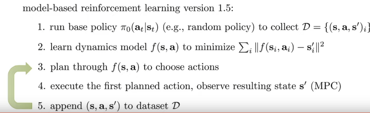
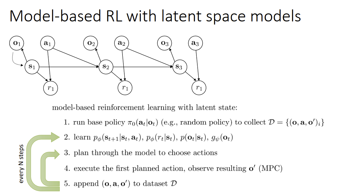
Why Model-based methods? Because if we know the transition function f(st,at)=P(st+1st,at)f(s_t, a_t) = \mathbb{P}_{(s_{t+1}|s_t,a_t)} then we can use trajectory planning ⇒ So we can learn f(st,at)f(s_t,a_t) from data
📌
Model-based RL can be prone to error in distribution mismatch ⇒ very like behavior cloning because when planned trajectory queries out-of-sample states, then f()f(\cdot) is likely to be wrong

NPC

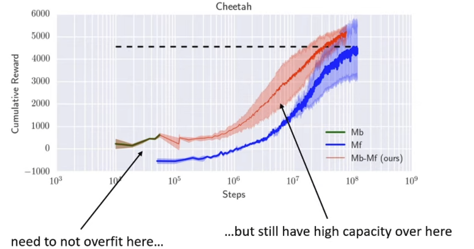
Performance Gap Issue

We want good exploration to gather more data to address the distribution shift, but with a not-so-good early model we cannot deploy good exploration techniques

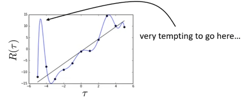
Basically the model early on overfits an function approximator and the exploration policy is stuck on a local minima / maxima

Uncertainty Estimation

Uncertainty estimation helps us reduce performance gap.

Under this trick, the expectation of reward under high-variance prediction is very low, even though the mean is the same

However:

  1. We still need exploration to get better model
  1. Expected value is not the same as pessimistic value

But how to build it?

  1. Use NN?
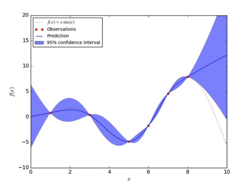
    1. Cannot express uncertainty of unseen data accurately ⇒ when querying out-of-sample data, the uncertainty output is arbitrary
    1. “The model is certain about data, but we are not certain about the model”
  1. Estimate Model Uncertainty
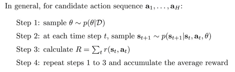
    1. Estimate arg maxθlogP(θD)=arg maxθlogP(Dθ)\argmax_\theta \log \mathbb{P}(\theta|D) = \argmax_\theta \log \mathbb{P}(D|\theta)
    1. Can we instead estimate the distribution P(θD)\mathbb{P}(\theta|D)?
      1. We can use this to get a posterior distribution over the next state
        1. p(st+1st,at,θ)p(θD)dθ\int p(s_{t+1}|s_t,a_t,\theta) p(\theta|D) d\theta
      1. Bayesian Neural Nets
        1. Every weight, instead of being a number, is a distribution
        1. But it’s difficult to join parameters into a single distribution
        1. So we do approximation
          1. p(θD)=ip(θiD)p(\theta|D) = \prod_i p(\theta_i|D)
            1. Very Crude approximation
          1. p(θiD)=N(μi,σi2)p(\theta_i|D) = N(\mu_i, \sigma_i^2)
            1. Instead of learning numerical value learn mean value and std/variance
          1. Bllundell et al. Weight Uncertainty in Neural Networks
          1. Gal et al. Concrete Dropout
  1. Bootstrap Ensembles
    1. Train several different neural nets and bootstrap samples(DiD_i sample with replacement from DD) to feed to those networks
      1. So each network learns slightly differently
      1. In theory each NN learns well on their own training data but makes different mistakes outside of training data
    1. Then estimate p(θD)1Niδ(θi)p(\theta|D) \approx \frac{1}{N} \sum_i \delta(\theta_i)
    1. p(st+1st,at,θ)p(θD)dθ1Nip(st+1st,at,θi)\int p(s_{t+1}|s_t,a_t,\theta) p(\theta|D) d\theta \approx \frac{1}{N} \sum_i p(s_{t+1}|s_t,a_t,\theta_i)
    1. Very crude approximation
      1. Because the number of models is usually small(expensive)
      1. But works
      1. Resampling with replacement is usually unnecessary, because SGD and random initialization usually makes the models sufficiently independent

With Complex Observations (images)

  1. High dimensionality with observation prediction model
    1. Redundancy
  1. Partial Observability

Can we seperately learn p(otst)p(o_t | s_t), which is high-dim but not dynamic, and p(st+1st,at)p(s_{t+1}|s_t,a_t), which is low-dim but dynamic?

Now we need to maximize

maxϕ1Ni=1Nt=1TE[logpϕ(st+1st,i,at,i)+logpϕ(ot,ist,i)]\max_\phi \frac{1}{N} \sum_{i=1}^N \sum_{t=1}^T \mathbb{E}[\log p_\phi(s_{t+1}|s_{t,i},a_{t,i}) + \log p_\phi (o_{t,i}|s_{t,i})]

Note that the expectation is conditioned on

(st,st+1)p(st,st+1o1:T,a1:T)(s_t,s_{t+1}) \sim p(s_t,s_{t+1}|o_{1:T},a_{1:T})

So can we learn an additional approximate posterior (encoder):

qψ(sto1:t,a1:t)q_\psi (s_t|o_{1:t},a_{1:t})

Also we have other choices:

  1. qψ(st,st+1o1:T,a1:T)q_\psi(s_t,s_{t+1}|o_{1:T},a_{1:T}) - full smoothing posterior
    1. most accurate
    1. most complicated to train
    1. Preferred when the state is less fully-observed
  1. qψ(stot)q_\psi (s_t | o_t)
    1. single-step encoder
    1. simplest but less accurate
    1. stochastic case requires variational inference
    1. Deterministic: qψ(stot)=δ(st=gψ(ot))q_\psi(s_t|o_t) = \delta(s_t = g_\psi(o_t))

To use uncertainty

Before uncertainty is introduced, we have (assuming st+1=f(st,at)s_{t+1} = f(s_t,a_t)

J(a1,,aH)=t=1Hr(st,at)J(a_1,\dots,a_H) = \sum_{t=1}^H r(s_t,a_t)

Now(With bootstrap):

J(a1,,aH)=1Ni=1Nt=1Hr(st,i,ai)J(a_1,\dots,a_H) = \frac{1}{N} \sum_{i=1}^N \sum_{t=1}^H r(s_{t,i},a_i)

Other options:

  1. Moment matching
  1. more complex posterior estimation with BNNs

Further Readings

  1. Classic
    1. Deisenroth et al. PILCO: A Model-Based and Data-Efficient Approach to Policy Search.
  1. Recent papers:
    1. Nagabandi et al. Neural Network Dynamics for Model-Based Deep Reinforcement Learning with Model-Free Fine-Tuning.
    1. Chua et al. Deep Reinforcement Learning in a Handful of Trials using Probabilistic Dynamics Models.
    1. Feinberg et al. Model-Based Value Expansion for Efficient Model-Free Reinforcement Learning.
    1. Buckman et al. Sample-Efficient Reinforcement Learning with Stochastic Ensemble Value Expansion.

Can we just backprop through policy / dynamics model?

📌
Generally No!
  1. Similar parameter sensitivity problems as shooting methods
    1. But no longer have convenient second order LQR-like method, because policy parameters couple all the time steps
  1. Similar problems to training long RNNs with BPTT
    1. Vanishing and exploding gradients

Let’s compare policy gradient:

θJ(θ)1Ni=1Nt=1Tθlogπθ(ai,tsi,t)Q^i,tπ\nabla_\theta J(\theta) \approx \frac{1}{N} \sum_{i=1}^N \sum_{t=1}^T \nabla_\theta \log \pi_\theta(a_{i,t}|s_{i,t})\hat{Q}_{i,t}^\pi

with backprop (pathwise) gradient:

θJ(θ)=t=1Tatθst+1at(t=t+1Trtst(t=t+2tstat1at1st1+stst1))\nabla_\theta J(\theta) = \sum_{t=1}^T \frac{\partial a_t}{\partial \theta} \frac{\partial s_{t+1}}{\partial a_t}(\sum_{t'=t+1}^T \frac{\partial r_{t'}}{\partial s_{t'}}(\prod_{t'' = t+2}^{t'} \frac{\partial s_{t''}}{\partial a_{t''-1}}\frac{\partial a_{t''-1}}{\partial s_{t''-1}}+\frac{\partial s_{t''}}{\partial s_{t''-1}}))

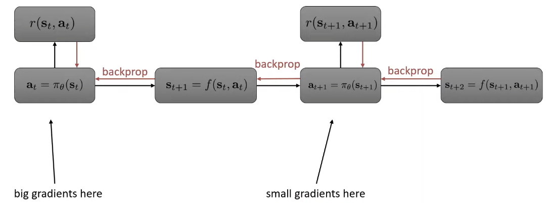
Policy gradient might be more stable (if enough samples are used) because it does not require multiplying many Jacobians

Parmass et al. “18: PIPP: Flexible Model-Based Policy Search Robust to the Curse of Chaos”

It we use policy gradient to backprop through our model dynamics model, there would still be a problem (although generating samples does not require interacting with physical world or simulator)

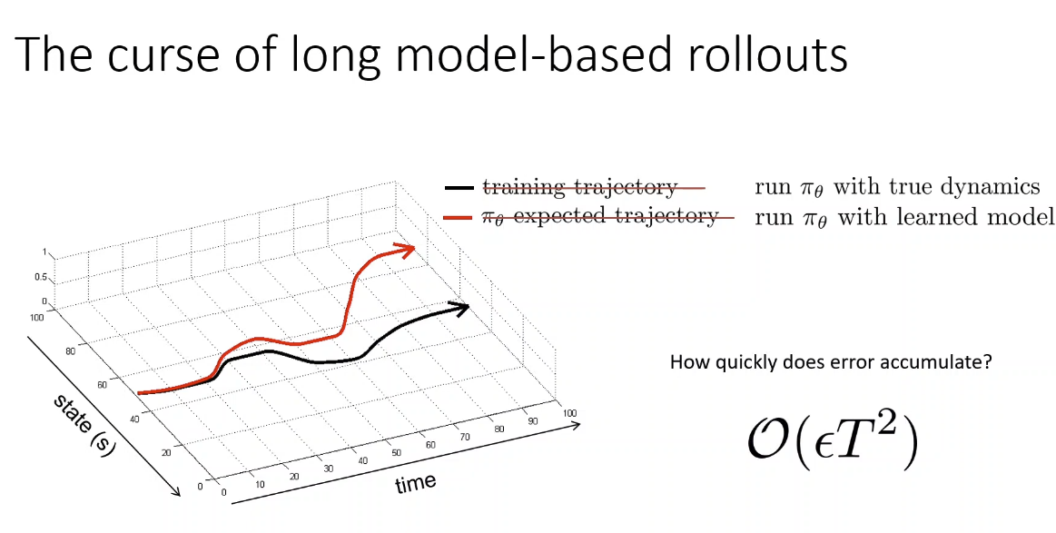
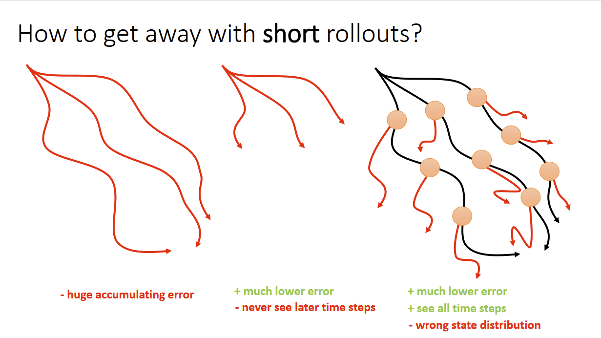
Left: Open-loop planning with long rollouts; Middle: Open-loop planning with shorter rollouts; Right: Collect real-world data from current policy and do short rollouts planning with data sampled from real distribution

But this does not solve the problem because the point of using model-based RL is being sample efficient and using sampled real world data and do short-rollout open-loop planning restrict how much we can change our policy.

Model-based RL with Policies

📌
Question is how to use the model’s predictions? fit Q functions or Value functions or what?
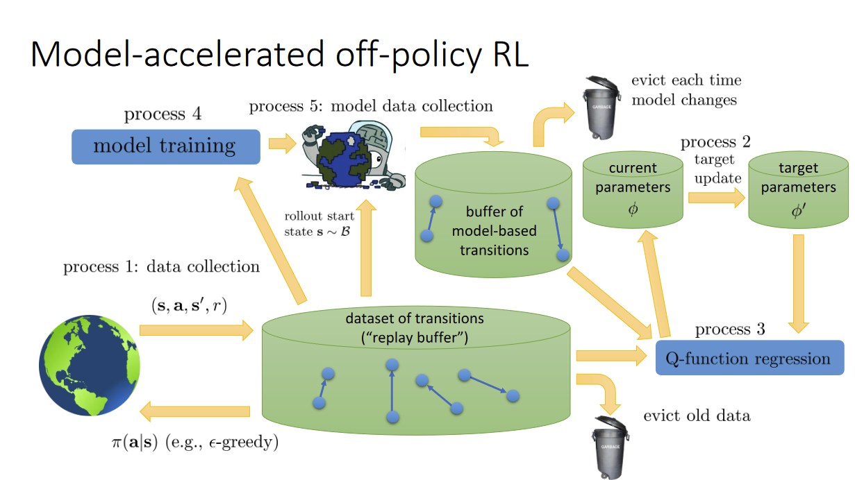
  1. Model-Based Acceleration (MBA)
    1. Gu et al. Continuous deep Q-learning with model-based acceleration. ‘16
  1. Model-Based Value Expansion (MVE)
    1. Feinberg et al. Model-based value expansion. ’18
  1. Model-Based Policy Optimization (MBPO)
    1. Janner et al. When to trust your model: model-based policy optimization. ‘19
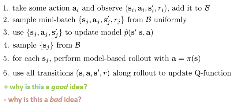
Good Idea:

  1. Sample Efficient

Bad Idea:

  1. Additional Source of bias if model is not correct
    1. Reduce this by using ensemble methods
  1. If not seen states before then we still cannot perform valid action

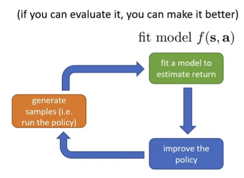
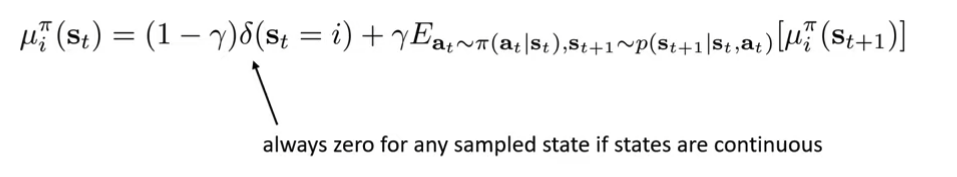
Multi-step Models and Successor Representations

📌
The job of the model is to evaluate the policy
Vπ(st)=t=tγttEp(ststEatst)[r(st,at)]=t=tγttEp(stst)[r(st)]=t=tγttsp(st=sst)r(s)=s(t=tγttp(st=sst))undefinedAdd (1γ) term to the front makes it pπ(sfuture=sst)r(s)\begin{split} V^\pi(s_t) &= \sum_{t=t'}^\infin \gamma^{t'-t} \mathbb{E}_{p(s_{t'}|s_t} \mathbb{E}_{a_{t'}|s_{t'})}[r(s_{t'},a_{t'})] \\ &= \sum_{t=t'}^\infin \gamma^{t' - t} \mathbb{E}_{p(s_{t'}|s_t)}[r(s_{t'})] \\ &= \sum_{t = t'}^\infin \gamma^{t'-t} \sum_s p(s_{t'} = s|s_t)r(s) \\ &= \sum_s \underbrace{(\sum_{t=t'}^\infin \gamma^{t' - t} p(s_{t'} = s | s_t))}_{\mathclap{\text{Add $(1-\gamma)$ term to the front makes it $p_\pi(s_{future}=s|s_t)$}}} r(s) \end{split}
pπ(sfuture=sst)=(1γ)t=tγttp(st=sst)p_\pi(s_{future}=s|s_t) = (1-\gamma)\sum_{t=t'}^\infin \gamma^{t' - t} p(s_{t'} = s | s_t)

Therefore

Vπ(st)=11γspπ(sfuture=sst)r(s)undefinedμπ(st)rV^\pi(s_t) = \frac{1}{1-\gamma} \underbrace{\sum_s p_\pi(s_{future}=s|s_t) r(s)}_{\mathclap{\mu^\pi(s_t)^\top \vec{r}}}

Where

μiπ=pπ(sfuture=sist)\mu_i^\pi = p_\pi(s_{future} = s_i|s_t)

is the “successor representation”

Dayan Improving Generalization for Temporal Difference Learning: The Successor Representation, 1993.

μiπ(st)=(1γ)t=tγttp(st=ist)=(1γ)δ(st=i)+γEatπ(atst),st+1p(st+1st,at)[μiπ(st+1]\begin{split} \mu_i^\pi(s_t) &= (1-\gamma) \sum_{t'=t}^\infin \gamma^{t'-t} p(s_{t'} = i | s_t) \\ &= (1-\gamma)\delta(s_t = i) + \gamma \mathbb{E}_{a_t \sim \pi(a_t|s_t), s_{t+1} \sim p(s_{t+1}|s_t,a_t)}[\mu_i^\pi(s_{t+1}] \end{split}

Hmm…looks like a bellman backup with “reward” r(st)=1γδ(st=i)r(s_t) = 1-\gamma \delta(s_t = i)

But issues:

  1. Not clear if learning successor representation is easier than model-free RL
  1. how to scale to large state spaces?
  1. How to extend to continuous state spaces?

To scale to large state spaces, use successor feature of sts_t

ψjπ(st)=sμsπ(st)ϕj(s)=μπ(st)ϕj\psi_j^\pi(s_t) = \sum_s \mu_s^\pi(s_t)\phi_j(s) = \mu_\pi(s_t)^\top \vec{\phi}_j

If we can express the reward function as combination of features of state s

r(s)=jϕj(s)wj=ϕ(s)wr(s) = \sum_j \phi_j(s) w_j = \phi(s)^\top w

Turns out we can express the value function as

Vπ(st)=ψπ(st)w=jμπ(st)ϕjw=μπ(st)jϕjw=μπ(st)rV^\pi(s_t) = \psi^\pi(s_t)^\top w = \sum_j \mu^\pi(s_t)^\top \vec{\phi}_j w = \mu^\pi(s_t)^\top \sum_j \vec{\phi}_j w = \mu^\pi(s_t)^\top \vec{r}

The dimensionality of ϕ\phi and ψ\psi would be a lot lower than the dimension of possible states

Can also construct a Q-function like version

ψjπ(st,at)=ϕj(st)+γEst+1p(st+1st,at),at+1π(at+1st+1)[ψjπ(st+1,at+1)]\psi_j^\pi(s_t,a_t) = \phi_j(s_t) + \gamma \mathbb{E}_{s_{t+1} \sim p(s_{t+1}|s_t,a_t), a_{t+1} \sim \pi(a_{t+1}|s_{t+1})}[\psi_j^\pi(s_{t+1},a_{t+1})]
Qπ(st,at)ψπ(st,at)wQ^\pi(s_t,a_t) \approx \psi^\pi(s_t,a_t)^\top w

(when r(s)=ϕ(s)wr(s) = \phi(s)^\top w)

Using Successor Features

  1. Recover a Q-function very quickly
    1. Train ψπ(st,at)\psi^\pi(s_t,a_t) via Bellman backups
    1. Get some reward samples {si,ri}\{s_i, r_i \}
    1. Get warg minwiϕ(si)wri2w \leftarrow \argmin_w \sum_i ||\phi(s_i)^\top w - r_i||^2
    1. Recover Qπ(st,at)ψπ(st,at)wQ^\pi(s_t,a_t) \approx \psi^\pi(s_t,a_t)^\top w
      1. π(s)=arg maxaψπ(s,a)w\pi’(s) = \argmax_a \psi^\pi(s,a)^\top w
        1. This is only equivalent to one step of policy iteration because Q is with respect to the actor
  1. Recover many Q-function
    1. Train ψπk(st,at)\psi^{\pi_k}(s_t,a_t) for many policies πk\pi_k via Bellman backups
    1. Get some reward samples {si,ri}\{s_i, r_i \}
    1. Get warg minwiϕ(si)wri2w \leftarrow \argmin_w \sum_i ||\phi(s_i)^\top w - r_i||^2
    1. Recover Qπk(st,at)ψπk(st,at)wQ^{\pi_k}(s_t,a_t) \approx \psi^{\pi_k}(s_t,a_t)^\top w for every πk\pi_k
      1. π(s)=arg maxamaxkψπk(s,a)w\pi’(s) = \argmax_a \max_k \psi^{\pi_k}(s,a)^\top w
        1. This is only equivalent to one step of policy iteration because Q is with respect to the actor
        1. Finding to highest reward policy in each state

Continuous Successor Representations (C-Learning)

🧙🏽‍♂️
So can we just frame successor representation as classification?
pπ(F=1undefinedmeans sfuture is a future state under πst,at,sfuture)=pπ(sfuturest,at)pπ(sfuturest,at)+pπ(sfuture)p^\pi(\underbrace{F=1}_{\mathclap{\text{means $s_{future}$ is a future state under $\pi$}}}|s_t,a_t,s_{future}) = \frac{p^\pi(s_{future}|s_t,a_t)}{p^\pi(s_{future}|s_t,a_t)+p^\pi(s_{future})}

Positive set during training:

D+pπ(sfuturest,at)D_+ \sim p^\pi(s_{future}|s_t,a_t)

Negative set just pulled randomly.

To train (On-policy algorithm, can also derive an off-policy algorithm that is also very efficient):

  1. Sample spπ(s)s\sim p^\pi(s) ⇒ run policy, sample from trajectories
  1. Sample spπ(sfuturest,at)s \sim p^\pi(s_{future}|s_t,a_t) ⇒ pick positive future pairs
  1. Update pπ(F=1st,at,s)p^\pi(F=1|s_t,a_t,s) using SGD with cross entropy loss

Eysenbach, Salakhutdinov, Levine. C-Learning: Learning to Achieve Goals via Recursive Classification. 2020.