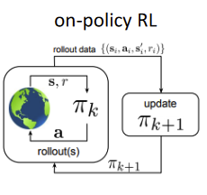
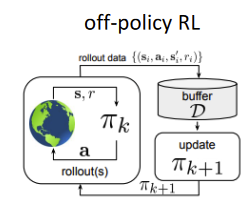
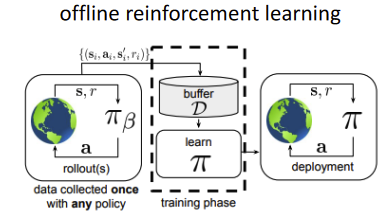
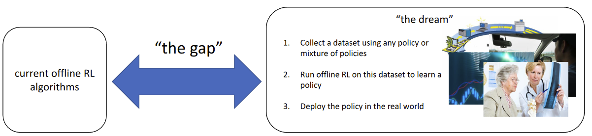
Huge gap in DL and DRL ⇒ supervised learning has tons of data! Formally:
D = { ( s i , a i , s i ′ , r i ) } s ∼ d π β ( s ) a ∼ π β ( a ∣ s ) r ← r ( s , a ) D = \{ (s_i,a_i,s_i',r_i) \} \\
s \sim d^{\pi_\beta}(s) \\
a \sim \pi_\beta(a|s) \\
r \leftarrow r(s,a) D = {( s i , a i , s i ′ , r i )} s ∼ d π β ( s ) a ∼ π β ( a ∣ s ) r ← r ( s , a ) π β \pi_\beta π β Off-Policy Evaluation (OPE) Given D D D J ( π β ) J(\pi_\beta) J ( π β ) Offline Reinforcement Learning Given D D D best possible policy π θ \pi_\theta π θ How is this even possible?
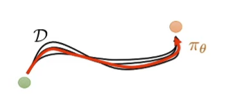
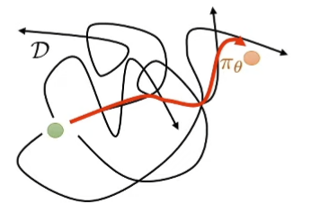
Find the “good stuff” in a dataset full of good and bad behaviors Generalization: Good behavior in one place may suggest good behavior in another place “Stitching”: Parts of good behaviors (even badly-performed parts can have good behaviors) can be recombined Bad intuition: It’s like imitation learningThough it can be shown to be provably better than imitation learning even with optimal data, under some structural assumptions ⇒ Kumar, Hong, Singh, Levine. Should I Run Offline Reinforcement Learning or Behavioral Cloning? Better Intuition: Get order from chaose.g. Get object from a drawer ⇒ Singh, Yu, Yang, Zhang, Kumar, Levine. COG: Connecting New Skills to Past Experience with Offline Reinforcement Learning.
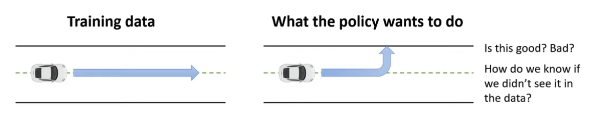
Behavior Cloning “Stiching” What can go wrong if we just use off-policy RL (on data collected by other agents)?
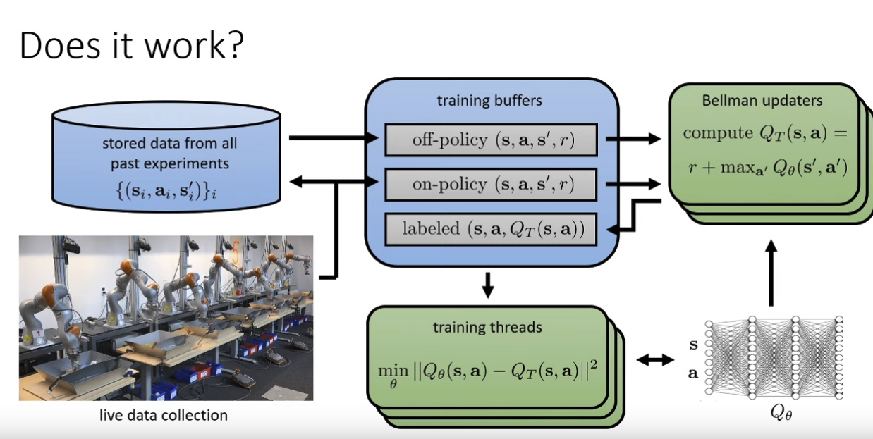
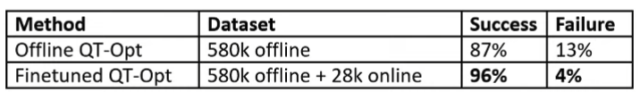
Kalashnikov, Irpan, Pastor, Ibarz, Herzong, Jang, Quillen, Holly, Kalakrishnan, Vanhoucke, Levine. QT-Opt: Scalable Deep Reinforcement Learning of Vision-based Robotic Manipulation Skills So it works in practice, but seems like a huge GAP between not-fine-tuned and fine-tuned result?
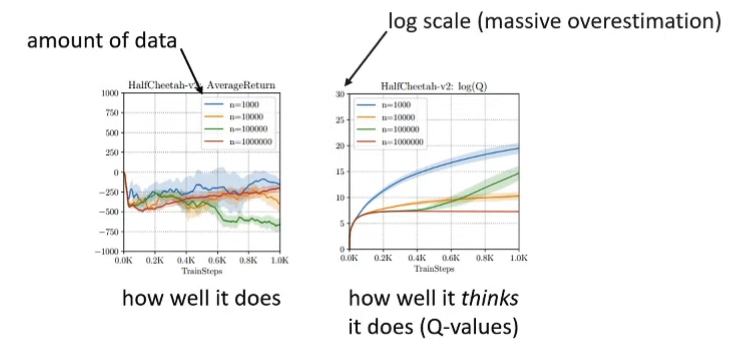
Kumar, Fu, Tucker, Levine. Stabilizing Off-Policy Q-Learning via Bootstrapping Error Reduction. NeurIPS ‘19 Q-function overfitting with an off-policy actor-critic algorithm Fundamental Problem: Counterfactual queries Online RL algorithms don’t have to handle this because they can simply try this action and see what happens ⇒ not possible for offline policies
Offline RL methods must somehow account for these unseen (”out-of-distribution”) actions , ideally in a safe way
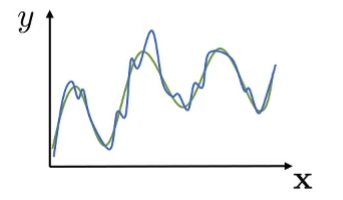
Distribution Shift In a supervised learning setting, we want to perform empirical risk minimization (ERM):
θ ← arg min θ E x ∼ p ( x ) , y ∼ p ( y ∣ x ) [ ( f θ ( x ) − y ) 2 ] \theta \leftarrow \argmin_\theta \mathbb{E}_{x \sim p(x), y\sim p(y|x)} [(f_\theta(x)-y)^2] θ ← θ arg min E x ∼ p ( x ) , y ∼ p ( y ∣ x ) [( f θ ( x ) − y ) 2 ] Given some x ∗ x^* x ∗
E x ∼ p ( x ) , y ∼ p ( y ∣ x ) [ ( f θ ( x ) − y ) 2 ] is low(since distribution is same as training set) E x ∼ p ˉ ( x ) , y ∼ p ( y ∣ x ) [ ( f θ ( x ) − y ) 2 ] is generally not if p ˉ ( x ) ≠ p ( x ) \mathbb{E}_{x \sim p(x), y\sim p(y|x)} [(f_\theta(x)-y)^2] \text{ is low(since distribution is same as training set)} \\
\mathbb{E}_{x \sim \bar{p}(x), y \sim p(y|x)} [(f_\theta(x)-y)^2] \text{ is generally not if $\bar{p}(x) \ne p(x)$} E x ∼ p ( x ) , y ∼ p ( y ∣ x ) [( f θ ( x ) − y ) 2 ] is low(since distribution is same as training set) E x ∼ p ˉ ( x ) , y ∼ p ( y ∣ x ) [( f θ ( x ) − y ) 2 ] is generally not if p ˉ ( x ) = p ( x ) Yes, neural nets generalize well ⇒ but is is well enough?
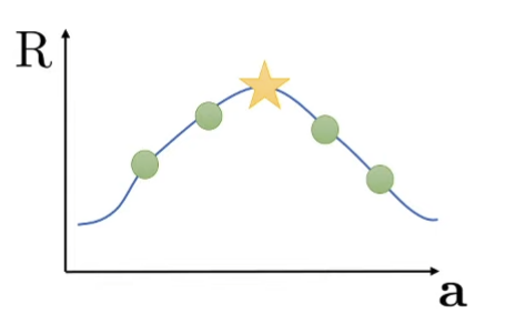
If we pick x ∗ ← arg max x f θ ( x ) x^* \leftarrow \argmax_x f_\theta(x) x ∗ ← arg max x f θ ( x )
Blue curve is the fitted and the green is the actual When we choose argmax we are probably including a huge positive noise!
Q-Learning Actor-Critic with Distribution Shift Q-objective:
min Q E ( s , a ) ∼ π β ( s , a ) [ ( Q ( s , a ) − y ( s , a ) ) 2 ] \min_{Q} \mathbb{E}_{(s,a) \sim \pi_\beta(s,a)}[(Q(s,a)-y(s,a))^2] Q min E ( s , a ) ∼ π β ( s , a ) [( Q ( s , a ) − y ( s , a ) ) 2 ] The function approximates:
Q ( s , a ) ← r ( s , a ) + E a ′ ∼ π n e w [ Q ( s ′ , a ′ ) ] Q(s,a) \leftarrow r(s,a) + \mathbb{E}_{a' \sim \pi_{new}}[Q(s',a')] Q ( s , a ) ← r ( s , a ) + E a ′ ∼ π n e w [ Q ( s ′ , a ′ )] The distribution shift problem kicks in when
π n e w ≠ π β \pi_{new} \ne \pi_\beta π n e w = π β And even worse,
π n e w = arg max π E a ∼ π ( a ∣ s ) [ Q ( s , a ) ] \pi_{new} = \argmax_\pi \mathbb{E}_{a \sim \pi(a|s)} [Q(s,a)] π n e w = π arg max E a ∼ π ( a ∣ s ) [ Q ( s , a )] Online RL Setting (Sample “optimal” and find error in our approximation)
Offline Setting (No way to find error in our approximation)
🧙🏽♂️
Existing Challenges with sampling error and function approximation error in standard RL become much more severe in offline RL
Batch RL via Important Sampling (Traditional Offline Algorithms) Importance Sampling:
∇ θ J ( θ ) ≈ 1 N ∑ i = 1 N π θ ( τ i ) π β ( τ i ) undefined importance weight ∑ t = 0 T ∇ θ γ t log π θ ( a t , i ∣ s t , i ) Q ^ ( s t , i , a t , i ) \nabla_\theta J(\theta) \approx \frac{1}{N} \sum_{i=1}^N \underbrace{\frac{\pi_\theta(\tau_i)}{\pi_\beta(\tau_i)}}_{\mathclap{\text{importance weight}}} \sum_{t=0}^T \nabla_\theta \gamma^t \log \pi_\theta(a_{t,i}|s_{t,i})\hat{Q}(s_{t,i},a_{t,i}) ∇ θ J ( θ ) ≈ N 1 i = 1 ∑ N importance weight π β ( τ i ) π θ ( τ i ) t = 0 ∑ T ∇ θ γ t log π θ ( a t , i ∣ s t , i ) Q ^ ( s t , i , a t , i ) Where the importance weight, is exponential in T
π θ ( τ ) π β ( τ ) = p ( s 1 ) ∏ t p ( s t + 1 ∣ s t , a t ) π θ ( a t ∣ s t ) p ( s 1 ) ∏ t p ( s t + 1 ∣ s t , a t ) π β ( a t ∣ s t ) ∈ O ( e T ) \frac{\pi_\theta(\tau)}{\pi_\beta(\tau)} = \frac{p(s_1) \prod_t p(s_{t+1}|s_t,a_t)\pi_\theta(a_t|s_t)}{p(s_1)\prod_t p(s_{t+1}|s_t,a_t) \pi_\beta(a_t|s_t)} \in O(e^T) π β ( τ ) π θ ( τ ) = p ( s 1 ) ∏ t p ( s t + 1 ∣ s t , a t ) π β ( a t ∣ s t ) p ( s 1 ) ∏ t p ( s t + 1 ∣ s t , a t ) π θ ( a t ∣ s t ) ∈ O ( e T ) Can we fix this?
∇ θ J ( θ ) ≈ 1 N ∑ i = 1 N ∑ t = 0 T ( ∏ t ′ = 0 t − 1 π θ ( a t ′ , i ∣ s t ′ , i ) π β ( a t ′ , i ∣ s t ′ , i ) ) undefined accounts for difference in probability of landing in s t , i ∇ θ γ t log π θ ( a t , i ∣ s t , i ) ( ∏ t ′ = t T π θ ( a t ′ , i ∣ s t ′ , i ) π β ( a t ′ , i ∣ s t ′ , i ) ) undefined accounts for incorrect Q ^ ( s t , i , a t , i ) Q ^ ( s t , i , a t , i ) \nabla_\theta J(\theta) \approx \frac{1}{N} \sum_{i=1}^N \sum_{t=0}^T \underbrace{(\prod_{t'=0}^{t-1} \frac{\pi_\theta(a_{t',i}|s_{t',i})}{\pi_\beta(a_{t',i}|s_{t',i})})}_{\mathclap{\text{accounts for difference in probability of landing in $s_{t,i}$}}} \nabla_\theta \gamma^t \log \pi_\theta(a_{t,i}|s_{t,i}) \underbrace{(\prod_{t'=t}^T\frac{\pi_\theta(a_{t',i}|s_{t',i})}{\pi_\beta(a_{t',i}|s_{t',i})}) }_{\mathclap{\text{accounts for incorrect $\hat{Q}(s_{t,i},a_{t,i})$}}}\hat{Q}(s_{t,i},a_{t,i}) ∇ θ J ( θ ) ≈ N 1 i = 1 ∑ N t = 0 ∑ T accounts for difference in probability of landing in s t , i ( t ′ = 0 ∏ t − 1 π β ( a t ′ , i ∣ s t ′ , i ) π θ ( a t ′ , i ∣ s t ′ , i ) ) ∇ θ γ t log π θ ( a t , i ∣ s t , i ) accounts for incorrect Q ^ ( s t , i , a t , i ) ( t ′ = t ∏ T π β ( a t ′ , i ∣ s t ′ , i ) π θ ( a t ′ , i ∣ s t ′ , i ) ) Q ^ ( s t , i , a t , i ) Classic Advanced Policy Gradient RL completely strips away the first product term ⇒ assuming that the new policy π θ \pi_\theta π θ π β \pi_\beta π β
We can estimate
Q ^ ( s t , i , a t , i ) = E π θ [ ∑ t ′ = t T γ t ′ − t r t ′ ] ≈ ∑ t ′ = t T γ t ′ − t r t ′ , i \hat{Q}(s_{t,i},a_{t,i}) = \mathbb{E}_{\pi_\theta}[\sum_{t'=t}^T \gamma^{t'-t} r_{t'}] \approx \sum_{t'=t}^T \gamma^{t'-t} r_{t',i} Q ^ ( s t , i , a t , i ) = E π θ [ t ′ = t ∑ T γ t ′ − t r t ′ ] ≈ t ′ = t ∑ T γ t ′ − t r t ′ , i We can simplify the portion (using the fact that future actions don’t affect current reward)
( ∏ t ′ = t T π θ ( a t ′ , i ∣ s t ′ , i ) π β ( a t ′ , i ∣ s t ′ , i ) ) Q ^ ( s t , i , a t , i ) = ∑ t ′ = t T ( ∏ t ′ ′ = t T π θ ( a t ′ ′ , i ∣ s t ′ ′ , i ) π β ( a t ′ ′ , i ∣ s t ′ ′ , i ) ) Q ^ ( s t , i , a t , i ) ≈ ∑ t ′ = t T ( ∏ t ′ ′ = t t ′ π θ ( a t ′ ′ , i ∣ s t ′ ′ , i ) π β ( a t ′ ′ , i ∣ s t ′ ′ , i ) ) Q ^ ( s t ′ , i , a t ′ , i ) (\prod_{t'=t}^T\frac{\pi_\theta(a_{t',i}|s_{t',i})}{\pi_\beta(a_{t',i}|s_{t',i})})\hat{Q}(s_{t,i},a_{t,i}) = \sum_{t'=t}^T(\prod_{t''=t}^T\frac{\pi_\theta(a_{t'',i}|s_{t'',i})}{\pi_\beta(a_{t'',i}|s_{t'',i})})\hat{Q}(s_{t,i},a_{t,i}) \approx \sum_{t'=t}^T(\prod_{t''=t}^{t'}\frac{\pi_\theta(a_{t'',i}|s_{t'',i})}{\pi_\beta(a_{t'',i}|s_{t'',i})})\hat{Q}(s_{t',i},a_{t',i}) ( t ′ = t ∏ T π β ( a t ′ , i ∣ s t ′ , i ) π θ ( a t ′ , i ∣ s t ′ , i ) ) Q ^ ( s t , i , a t , i ) = t ′ = t ∑ T ( t ′′ = t ∏ T π β ( a t ′′ , i ∣ s t ′′ , i ) π θ ( a t ′′ , i ∣ s t ′′ , i ) ) Q ^ ( s t , i , a t , i ) ≈ t ′ = t ∑ T ( t ′′ = t ∏ t ′ π β ( a t ′′ , i ∣ s t ′′ , i ) π θ ( a t ′′ , i ∣ s t ′′ , i ) ) Q ^ ( s t ′ , i , a t ′ , i ) But this is still exponential in T T T
🧙🏽♂️
To avoid exponentially exploding importance weights, we must use value function estimation !
The Doubly Robust Estimator Jiang, N. and Li, L. (2015). Doubly robust off-policy value evaluation for reinforcement learning V π θ ( s 0 ) ≈ ∑ t = 0 T ( ∏ t ′ = 0 t π θ ( a t ′ ∣ s t ′ ) π β ( a t ′ ∣ s t ′ ) ) γ t r t = ∑ t = 0 T ( ∏ t ′ = 0 t ρ t ′ ) γ t r t = ρ 0 r 0 + ρ 0 γ ρ 1 r 1 + ρ 0 γ ρ 1 γ ρ 2 r 2 + … = ρ 0 ( r 0 + γ ( ρ 1 ( r 1 + . . . ) ) ) = V ˉ T \begin{split}
V^{\pi_\theta}(s_0) &\approx \sum_{t=0}^T (\prod_{t'=0}^t \frac{\pi_\theta(a_{t'}|s_{t'})}{\pi_\beta(a_{t'}|s_{t'})})\gamma^t r_t \\
&= \sum_{t=0}^T(\prod_{t'=0}^t \rho_{t'}) \gamma^t r_t \\
&= \rho_0 r_0 + \rho_0\gamma\rho_1r_1 + \rho_0\gamma \rho_1 \gamma \rho_2 r_2 + \dots \\
&=\rho_0(r_0 + \gamma(\rho_1(r_1+...))) \\
&=\bar{V}^T
\end{split} V π θ ( s 0 ) ≈ t = 0 ∑ T ( t ′ = 0 ∏ t π β ( a t ′ ∣ s t ′ ) π θ ( a t ′ ∣ s t ′ ) ) γ t r t = t = 0 ∑ T ( t ′ = 0 ∏ t ρ t ′ ) γ t r t = ρ 0 r 0 + ρ 0 γ ρ 1 r 1 + ρ 0 γ ρ 1 γ ρ 2 r 2 + … = ρ 0 ( r 0 + γ ( ρ 1 ( r 1 + ... ))) = V ˉ T We notice a recursion relationship:
V ˉ T + 1 − t = ρ t ( r t + γ V ˉ T − t ) \bar{V}^{T+1-t} = \rho_t(r_t + \gamma \bar{V}^{T-t}) V ˉ T + 1 − t = ρ t ( r t + γ V ˉ T − t ) Bandit case of doubly robust estimation:
V D R ( s ) = V ^ ( s ) + ρ ( s , a ) ( r s , a − Q ^ ( s , a ) ) V_{DR}(s) = \hat{V}(s) + \rho(s,a)(r_{s,a} - \hat{Q}(s,a)) V D R ( s ) = V ^ ( s ) + ρ ( s , a ) ( r s , a − Q ^ ( s , a )) Doubly Robust Estimation:
V ˉ D R T + 1 − t = V ^ ( s t ) + ρ t ( r t + γ V ˉ D R T − t − Q ^ ( s t , a t ) ) \bar{V}_{DR}^{T+1-t} = \hat{V}(s_t) + \rho_t(r_t + \gamma \bar{V}_{DR}^{T-t} - \hat{Q}(s_t,a_t)) V ˉ D R T + 1 − t = V ^ ( s t ) + ρ t ( r t + γ V ˉ D R T − t − Q ^ ( s t , a t )) Marginalized Important Sampling In previous times we were trying to do importance sampling on action distributions ⇒ but it’s actually possible to do it on state distributions 🧙🏽♂️
Instead of using
∏ t π θ ( a t ∣ s t ) π β ( a t ∣ s t ) \prod_t \frac{\pi_\theta(a_t|s_t)}{\pi_\beta(a_t|s_t)} ∏ t π β ( a t ∣ s t ) π θ ( a t ∣ s t ) , estimate
w ( s , a ) = d π θ ( s , a ) d π β ( s , a ) w(s,a) = \frac{d^{\pi_\theta}(s,a)}{d^{\pi_\beta}(s,a)} w ( s , a ) = d π β ( s , a ) d π θ ( s , a ) How to determine w ( s , a ) w(s,a) w ( s , a )
Typically solve some kind of consistency condition e.g. (Zhang et al. GenDICE)d π β ( s ’ , a ’ ) w ( s ’ , a ’ ) = ( 1 − γ ) p 0 ( s ’ ) π θ ( a ’ ∣ s ’ ) + γ ∑ s , a π θ ( a ’ ∣ s ’ ) p ( s ’ ∣ s , a ) d π β ( s , a ) w ( s , a ) d^{\pi_\beta}(s’,a’)w(s’,a’) = (1-\gamma) p_0 (s’) \pi_\theta(a’|s’) + \gamma \sum_{s,a} \pi_\theta(a’|s’) p(s’|s,a) d^{\pi_\beta}(s,a) w(s,a) d π β ( s ’ , a ’ ) w ( s ’ , a ’ ) = ( 1 − γ ) p 0 ( s ’ ) π θ ( a ’∣ s ’ ) + γ ∑ s , a π θ ( a ’∣ s ’ ) p ( s ’∣ s , a ) d π β ( s , a ) w ( s , a ) Probability of seeing ( s ’ , a ’ ) (s’,a’) ( s ’ , a ’ ) s ’ s’ s ’ a ’ a’ a ’ s ’ s’ s ’ a ’ a’ a ’ Solving for w ( s , a ) w(s,a) w ( s , a )
Suggested Reading
Classic work on importance sampled policy gradients and return estimation:Precup, D. (2000). Eligibility traces for off-policy policy evaluation. Peshkin, L. and Shelton, C. R. (2002). Learning from scarce experience. Doubly robust estimators and other improved importance-sampling estimators:Jiang, N. and Li, L. (2015). Doubly robust off-policy value evaluation for reinforcement learning. Thomas, P. and Brunskill, E. (2016). Data-efficient off-policy policy evaluation for reinforcement learning. Analysis and theory:Thomas, P. S., Theocharous, G., and Ghavamzadeh, M. (2015). High-confidence off-policy evaluation. Marginalized importance sampling:Hallak, A. and Mannor, S. (2017). Consistent on-line off-policy evaluation. Liu, Y., Swaminathan, A., Agarwal, A., and Brunskill, E. (2019). Off-policy policy gradient with state distribution correction. Additional readings in our offline RL survey
Batch RL via Linear Fitted Value Functions How have people thought about it before? Extend existing ideas for approximate dynamic programming and Q-learning to offline setting Derive tractable solutions with simple (e.g., linear) function approximators Distribution Shift not a huge problem since value functions are relatively simple How are people thinking about it now?Derive approximate solutions with highly expressive function approximators (e.g., deep nets) The primary challenge turns out to be distributional shift
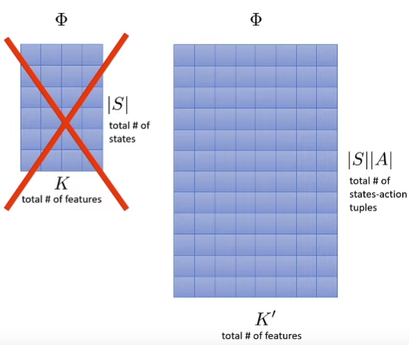
Assume we have a feature matrix
Φ ∈ R ∣ S ∣ × K \Phi \in \mathbb{R}^{|S| \times K} Φ ∈ R ∣ S ∣ × K where ∣ S ∣ |S| ∣ S ∣ K K K in feature space
Estimate the rewardΦ w r ≈ r \Phi w_r \approx r Φ w r ≈ r w r = ( Φ ⊤ Φ ) − 1 Φ ⊤ r ⃗ w_r = (\Phi^{\top} \Phi)^{-1} \Phi^{\top} \vec{r} w r = ( Φ ⊤ Φ ) − 1 Φ ⊤ r Estimate the transitionsΦ P Φ ≈ P π Φ \Phi P_{\Phi} \approx P^{\pi} \Phi Φ P Φ ≈ P π Φ P Φ P_\Phi P Φ ∈ R K × K \in \mathbb{R}^{K \times K} ∈ R K × K P ϕ = ( Φ ⊤ Φ ) − 1 Φ ⊤ P π Φ P_\phi = (\Phi^{\top} \Phi)^{-1} \Phi^{\top} P^{\pi} \Phi P ϕ = ( Φ ⊤ Φ ) − 1 Φ ⊤ P π Φ P π ∈ R ∣ S ∣ × ∣ S ∣ P^\pi \in \mathbb{R}^{|S| \times |S|} P π ∈ R ∣ S ∣ × ∣ S ∣ Estimate the value functionV π ≈ V Φ π = Φ w V V^{\pi} \approx V_{\Phi}^\pi = \Phi w_V V π ≈ V Φ π = Φ w V Solving for V π V^\pi V π P π P^\pi P π r r r V π = r + γ P Π V π V^\pi = r + \gamma P^\Pi V^\pi V π = r + γ P Π V π ( 1 − γ P π ) V π = r (1-\gamma P^\pi) V^\pi = r ( 1 − γ P π ) V π = r V π = ( I − γ P π ) − 1 r V^\pi = (I - \gamma P^\pi)^{-1}r V π = ( I − γ P π ) − 1 r w V = ( I − γ P Φ ) − 1 w r = ( Φ ⊤ Φ − γ Φ ⊤ P π Φ ) − 1 Φ ⊤ r ⃗ w_V = (I - \gamma P_\Phi)^{-1} w_r = (\Phi^\top \Phi-\gamma \Phi^\top P^\pi \Phi)^{-1} \Phi^\top \vec{r} w V = ( I − γ P Φ ) − 1 w r = ( Φ ⊤ Φ − γ Φ ⊤ P π Φ ) − 1 Φ ⊤ r But we don’t know P π P^\pi P π With samples introduced, we will change our feature matrix Φ ∈ R ∣ D ∣ × K \Phi \in \mathbb{R}^{|D| \times K} Φ ∈ R ∣ D ∣ × K And now we are going to replace P π Φ P^\pi \Phi P π Φ Φ ’ \Phi’ Φ’ Φ ’ i \Phi’_i Φ ’ i Φ i ’ = ϕ ( s i ’ ) \Phi_i’ = \phi(s_i’) Φ i ’ = ϕ ( s i ’ ) However, if we change policy, we no longer have P π P^\pi P π Also replace r ⃗ i = r ( s i , a i ) \vec{r}_i = r(s_i,a_i) r i = r ( s i , a i ) Everything else works exactly same, but only that we now have some sampling error Improve the policyπ ’ ( s ) ← G r e e d y ( Φ w V ) \pi’(s) \leftarrow Greedy(\Phi w_V) π ’ ( s ) ← G ree d y ( Φ w V )
Least Squares Policy Iteration (LSPI) 🧙🏽♂️
Replace LSTD with LSTDQ - LSTD but for Q functions
w Q = ( Φ ⊤ Φ − γ Φ ⊤ Φ ′ undefined Φ i ′ = ϕ ( s i ′ , π ( s i ′ ) ) ) − 1 Φ ⊤ r ⃗ w_Q = (\Phi^\top \Phi-\gamma \Phi^\top \underbrace{\Phi'}_{\mathclap{\Phi'_i = \phi(s_i',\pi(s_i'))}})^{-1} \Phi^\top \vec{r} w Q = ( Φ ⊤ Φ − γ Φ ⊤ Φ i ′ = ϕ ( s i ′ , π ( s i ′ )) Φ ′ ) − 1 Φ ⊤ r LSPI:
Compute w Q w_Q w Q π k \pi_k π k π k + 1 ( s ) = arg max a ϕ ( s , a ) w Q \pi_{k+1}(s) = \argmax_a \phi(s,a)w_Q π k + 1 ( s ) = arg max a ϕ ( s , a ) w Q Set Φ i ’ = ϕ ( s i ’ , π k + 1 ( s i ’ ) ) \Phi_i’ = \phi(s_i’, \pi_{k+1}(s_i’)) Φ i ’ = ϕ ( s i ’ , π k + 1 ( s i ’ ))
Problem:
Does not solve the distribution shift problem (in step 2 of argmax)
Policy Constraints Very old idea, generally only implement this would not work well Q ← r ( s , a ) + E a ′ ∼ π n e w [ Q ( s ′ , a ′ ) ] Q \leftarrow r(s,a) + \mathbb{E}_{a' \sim \pi_{new}}[Q(s',a')] Q ← r ( s , a ) + E a ′ ∼ π n e w [ Q ( s ′ , a ′ )] π n e w ( a ∣ s ) = arg max π E a ∼ π ( a ∣ s ) [ Q ( s , a ) ] s.t. D K L ( π , π β ) ≤ ϵ \pi_{new}(a|s) = \argmax_\pi \mathbb{E}_{a \sim \pi(a|s)}[Q(s,a)] \text{ s.t. } D_{KL}(\pi,\pi_\beta) \le \epsilon π n e w ( a ∣ s ) = π arg max E a ∼ π ( a ∣ s ) [ Q ( s , a )] s.t. D K L ( π , π β ) ≤ ϵ D K L ( π , π β ) D_{KL}(\pi, \pi_\beta) D K L ( π , π β )
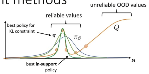
But not necessarily what we want So maybe instead we want to pose a “support constraint”
π ( a ∣ s ) ≥ 0 iff π β ( a ∣ s ) ≥ ϵ \pi(a|s) \ge 0 \text{ iff } \pi_\beta(a|s) \ge \epsilon π ( a ∣ s ) ≥ 0 iff π β ( a ∣ s ) ≥ ϵ Can approximate with Maximum Mean Discrepancy (MMD) significantly more complex to implement much closer to what we want
How to implement?
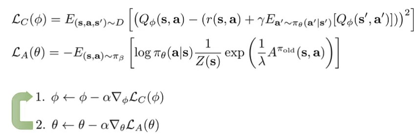
Implementing Implicit Policy Constraint in practice Modify the actor objectiveCommon objective θ ← arg max θ E s ∼ D [ E a ∼ π θ ( a ∣ s ) [ Q ( s , a ) ] ] \theta \leftarrow \argmax_\theta \mathbb{E}_{s \sim D} [\mathbb{E}_{a \sim \pi_\theta(a|s)}[Q(s,a)]] θ ← arg max θ E s ∼ D [ E a ∼ π θ ( a ∣ s ) [ Q ( s , a )]] D K L ( π , π β ) = E [ log π ( a ∣ s ) − log π β ( a ∣ s ) ] = − E π [ log π β ( a ∣ s ) ] − H ( π ) D_{KL}(\pi, \pi_\beta) = \mathbb{E}[\log \pi(a|s) - \log \pi_\beta (a|s)] = -\mathbb{E}_\pi[\log \pi_\beta(a|s)] - H(\pi) D K L ( π , π β ) = E [ log π ( a ∣ s ) − log π β ( a ∣ s )] = − E π [ log π β ( a ∣ s )] − H ( π ) So we can incorporate the KL divergence into the actor objective Use Lagrange Multiplierθ ← arg max θ E s ∼ D [ E a ∼ π θ ( a ∣ s ) [ Q ( s , a ) + λ log π β ( a ∣ s ) ] + λ H ( π ( a ∣ s ) ) ] \theta \leftarrow \argmax_\theta \mathbb{E}_{s \sim D} [\mathbb{E}_{a \sim \pi_\theta(a|s)}[Q(s,a) + \lambda \log \pi_\beta (a|s)]+\lambda H(\pi (a|s))] θ ← arg max θ E s ∼ D [ E a ∼ π θ ( a ∣ s ) [ Q ( s , a ) + λ log π β ( a ∣ s )] + λ H ( π ( a ∣ s ))] In practice we either solve the lagrange multiplier or treat it as hyper-parameter and tune it Modify the reward funcitonr ˉ ( s , a ) = r ( s , a ) − D ( π , π β ) \bar{r}(s,a) = r(s,a) - D(\pi, \pi_\beta) r ˉ ( s , a ) = r ( s , a ) − D ( π , π β ) Simple modification to directly penalize divergence Also accounts for future divergence (in later steps) Wu, Tucker, Nachum, Behavior Regularized Offline Reinforcement Learning. ‘19 Implicit Policy Constraint MethodsSolve for lagrangian condition of the KL constrained problem (straightforward to show via duality), we have π ∗ ( a ∣ s ) = 1 Z ( s ) π β ( a ∣ s ) exp ( 1 λ A π ( s , a ) ) \pi^*(a|s) = \frac{1}{Z(s)} \pi_\beta (a|s) \exp(\frac{1}{\lambda} A^\pi (s,a)) π ∗ ( a ∣ s ) = Z ( s ) 1 π β ( a ∣ s ) exp ( λ 1 A π ( s , a )) Peters et al. (REPS) Rawlik et al. (”psi-learning”) We can do this byApproximate via weighted max likelihood π n e w ( a ∣ s ) = arg max π E ( s , a ) ∼ π β undefined ( s , a ) ∼ D [ log π ( a ∣ s ) 1 Z ( s ) exp ( 1 λ A π o l d ( s , a ) ) undefined w ( s , a ) ] \pi_{new}(a|s) = \argmax_{\pi} \mathbb{E}_{\underbrace{(s,a) \sim \pi_\beta}_{(s,a) \sim D}} [\log \pi(a|s) \underbrace{\frac{1}{Z(s)} \exp(\frac{1}{\lambda} A^{\pi_{old}} (s,a)) }_{w(s,a)}] π n e w ( a ∣ s ) = arg max π E ( s , a ) ∼ D ( s , a ) ∼ π β [ log π ( a ∣ s ) w ( s , a ) Z ( s ) 1 exp ( λ 1 A π o l d ( s , a )) ] Imitating good actions “more”(determined by w ( s , a ) w(s,a) w ( s , a ) Problem: In order to get advantage values / target values we still need to query OOD actionsIf we choose λ \lambda λ 🧙🏽♂️
Can we avoid ALL OOD actions in the Q update?
Instead of doing
Q ( s , a ) ← r ( s , a ) + E a ′ ∼ π n e w [ Q ( s ′ , a ′ ) ] Q(s,a) \leftarrow r(s,a) + \mathbb{E}_{a' \sim \pi_{new}}[Q(s',a')] Q ( s , a ) ← r ( s , a ) + E a ′ ∼ π n e w [ Q ( s ′ , a ′ )] We can do:
Q ( s , a ) ← r ( s , a ) + V ( s ′ ) Q(s,a) \leftarrow r(s,a) + V(s') Q ( s , a ) ← r ( s , a ) + V ( s ′ ) But how do we fit this V ’ V’ V ’
V ← arg min V 1 N ∑ i = 1 N l ( V ( s i ) , Q ( s i , a i ) ) V \leftarrow \argmin_{V} \frac{1}{N} \sum_{i=1}^N l(V(s_i), Q(s_i, a_i)) V ← arg min V N 1 ∑ i = 1 N l ( V ( s i ) , Q ( s i , a i )) MSE Loss ( V ( s i ) − Q ( s i , a i ) ) 2 (V(s_i) - Q(s_i, a_i))^2 ( V ( s i ) − Q ( s i , a i ) ) 2 Problem is ⇒ the actions come from the exploration policy π β \pi_\beta π β π n e w \pi_{new} π n e w Gives us E a ∼ π β [ Q ( s , a ) ] \mathbb{E}_{a \sim \pi_\beta}[Q(s,a)] E a ∼ π β [ Q ( s , a )] Think about this:
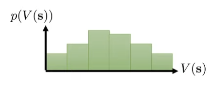
Distribution visualization of states We’ve probably seen only a bit or none of action in the “exact” same stateBut there might be very “similar” states that we execute action on ⇒ There’s not bins of states but distributions of states Can we use those “similar states” as extra data points for us to perform generalization on? But what if we use a “quantile” / “expectile” ⇒ expectile is like a quantile squaredUpper expectile / quantile is the best policy supported by the data
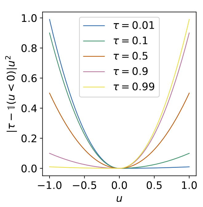
Implicit Q-Learning Expectile:
l 2 τ ( x ) = { ( 1 − τ ) x 2 if x > 0 τ x 2 otherwise l_2^\tau (x) = \begin{cases}
(1-\tau)x^2 &\text{if } x>0 \\
\tau x^2 &\text{otherwise}
\end{cases} l 2 τ ( x ) = { ( 1 − τ ) x 2 τ x 2 if x > 0 otherwise Intuition:
MSE penalizes positive and negative errors equally expectile penalizes positive and negative with different weights depending on τ ∈ [ 0 , 1 ] \tau \in [0,1] τ ∈ [ 0 , 1 ]
Weights given to positive and negative erros in expectile regression. Taken from IQL paper Formally, it could be shown that if we use
V ← arg min V E ( s , a ) ∼ D [ l 2 τ ( V ( s ) − Q ( s , a ) ) ] V \leftarrow \argmin_{V} \mathbb{E}_{(s,a) \sim D} [l_2^\tau(V(s)-Q(s,a))] V ← V arg min E ( s , a ) ∼ D [ l 2 τ ( V ( s ) − Q ( s , a ))] In practice, Q ( s , a ) Q(s,a) Q ( s , a )
Formally, we can prove that provided with a big enough τ \tau τ
V ( s ) ← max a ∈ Ω ( s ) Q ( s , a ) V(s) \leftarrow \max_{a \in \Omega(s)} Q(s,a) V ( s ) ← a ∈ Ω ( s ) max Q ( s , a ) Where
Ω ( s ) = { a : π β ( a ∣ s ) ≥ ϵ } \Omega(s) = \{a: \pi_\beta(a|s) \ge \epsilon \} Ω ( s ) = { a : π β ( a ∣ s ) ≥ ϵ } Kostrikov, Nair, Levine. Offline Reinforcement Learning with Implicit Q-Learning. ‘21 📌
Oh yes, that’s my postdoc’s paper (as the first author)! This is absolutely an amazing paper and he is absolutely an amazing person, also this is one of the papers I read for entering into Sergey’s group. I hope you get to check out this paper!
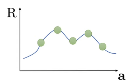
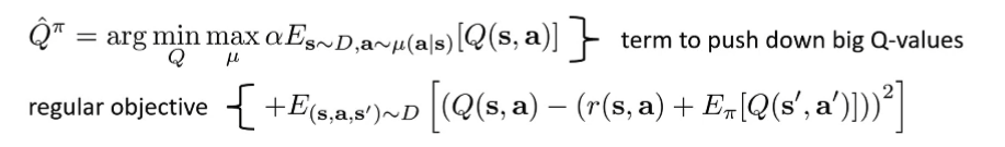
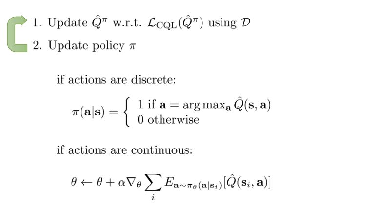
Conservative Q-Learning (CQL) Kumar, Zhou, Tucker, Levine. Conservative Q-Learning for Offline Reinforcement Learning Directly repair overestimated actions in the Q function
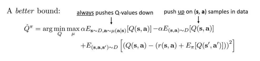
Intuition: Push down on areas that have errorneous high Q values We can formally show that Q ^ π ≤ Q π \hat{Q}^\pi \le Q^\pi Q ^ π ≤ Q π α \alpha α
But with this objective, we’re pressing down on actually “good” actions as well ⇒ so add additional terms that pushes up on good samples supported by data
No longer guarenteed that ∀ ( s , a ) Q ^ π ( s , a ) ≤ Q π ( s , a ) \forall (s,a) \hat{Q}^\pi (s,a) \le Q^\pi(s,a) ∀ ( s , a ) Q ^ π ( s , a ) ≤ Q π ( s , a ) But ∀ s ∈ D , E π ( a ∣ s ) [ Q ^ ( s , a ) ] ≤ E π ( a ∣ s ) [ Q π ( s , a ) ] \forall s\in D, \mathbb{E}_{\pi(a|s)}[\hat{Q}(s,a)] \le \mathbb{E}_{\pi(a|s)}[Q^\pi(s,a)] ∀ s ∈ D , E π ( a ∣ s ) [ Q ^ ( s , a )] ≤ E π ( a ∣ s ) [ Q π ( s , a )] In practice, we add a regularizer R ( μ ) R(\mu) R ( μ ) L C Q L ( Q ^ π ) L_{CQL}(\hat{Q}^\pi) L CQ L ( Q ^ π ) μ \mu μ
L C Q L ( Q ^ π ) = max μ { α E s ∼ D , a ∼ μ ( a ∣ s ) [ Q ^ π ( s , a ) ] − α E ( s , a ) ∼ D [ Q ( s , a ) ] } + E ( s , a , s ′ ) ∼ D [ ( Q ( s , a ) − ( r ( s , a ) + E [ Q ( s ′ , a ′ ) ] ) ) 2 ] L_{CQL}(\hat{Q}^\pi) = \max_{\mu} \{ \alpha\mathbb{E}_{s\sim D, a\sim \mu(a|s)}[\hat{Q}^\pi(s,a)] - \alpha \mathbb{E}_{(s,a) \sim D}[Q(s,a)] \} + \mathbb{E}_{(s,a,s') \sim D}[(Q(s,a) - (r(s,a)+\mathbb{E}[Q(s',a')]))^2] L CQ L ( Q ^ π ) = μ max { α E s ∼ D , a ∼ μ ( a ∣ s ) [ Q ^ π ( s , a )] − α E ( s , a ) ∼ D [ Q ( s , a )]} + E ( s , a , s ′ ) ∼ D [( Q ( s , a ) − ( r ( s , a ) + E [ Q ( s ′ , a ′ )]) ) 2 ] Common choice: R ( μ ) = E s ∼ D [ H ( μ ( ⋅ ∣ s ) ) ] R(\mu) = \mathbb{E}_{s \sim D} [H(\mu(\cdot | s))] R ( μ ) = E s ∼ D [ H ( μ ( ⋅ ∣ s ))]
⇒ Then μ ( a ∣ s ) ∝ exp [ Q ( s , a ) ] \mu(a|s) \propto \exp[Q(s,a)] μ ( a ∣ s ) ∝ exp [ Q ( s , a )] E a ∼ μ ( a ∣ s ) [ Q ( s , a ) ] = log ∑ a exp ( Q ( s , a ) ) \mathbb{E}_{a \sim \mu(a|s)}[Q(s,a)] = \log \sum_a \exp(Q(s,a)) E a ∼ μ ( a ∣ s ) [ Q ( s , a )] = log ∑ a exp ( Q ( s , a ))
For discrete actions, we can just calculate this log ∑ a exp ( Q ( s , a ) ) \log \sum_a \exp(Q(s,a)) log ∑ a exp ( Q ( s , a )) For continuous actions, use importance sampling to estimate E a ∼ μ ( a ∣ s ) [ Q ( s , a ) ] \mathbb{E}_{a \sim \mu (a|s)} [Q(s,a)] E a ∼ μ ( a ∣ s ) [ Q ( s , a )]
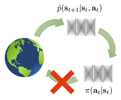
Model-based Offline RL What goes wrong when we cannot collect more data?
MOPO: Model-Based Offline Policy Optimization Yu*, Thomas*, Yu, Ermon, Zou, Levine, Finn, Ma. MOPO: Model-Based Offline Policy Optimization. ‘20
MOReL : Model-Based Offline Reinforcement Learning. ’20 (concurrent) “punish” the policy for exploiting
r ~ ( s , a ) = r ( s , a ) − λ u ( s , a ) \tilde{r}(s,a) = r(s,a) -\lambda u(s,a) r ~ ( s , a ) = r ( s , a ) − λ u ( s , a ) where u ( s , a ) u(s,a) u ( s , a )
u u u “Use ensemble as an error proxy for the uncertainty metric” ⇒ current method
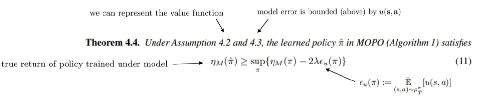
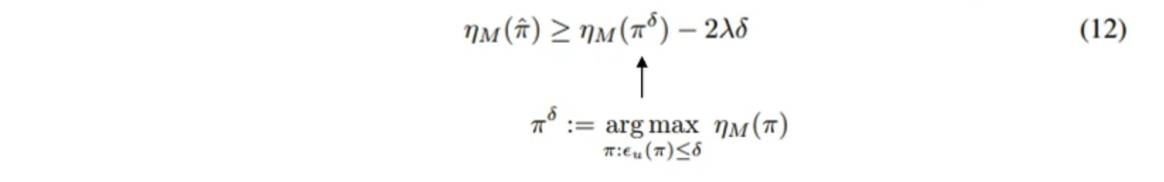
Theoretical analysis:
In particular, ∀ δ ≥ δ min \forall \delta \ge \delta_{\min} ∀ δ ≥ δ m i n
Some implications:
η M ( π ^ ) ≥ η M ( π B ) − 2 λ ϵ u ( π B ) \eta_M(\hat{\pi}) \ge \eta_M(\pi^{B})-2\lambda \epsilon_u(\pi^{B}) η M ( π ^ ) ≥ η M ( π B ) − 2 λ ϵ u ( π B ) We can do almost always better then the behavior(exploration) policy (since δ \delta δ π B \pi^B π B η M ( π ^ ) ≥ η M ( π ∗ ) − 2 λ ϵ u ( π ∗ ) \eta_M(\hat{\pi}) \ge \eta_M(\pi^*)-2\lambda \epsilon_u(\pi^*) η M ( π ^ ) ≥ η M ( π ∗ ) − 2 λ ϵ u ( π ∗ ) Quantifies the optimality “gap” in terms of model error
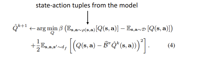
COMBO: Convervative Model-based RL Yu, Kumar, Rafailov, Rajeswaran, Levine, Finn. COMBO: Conservative Offline Model-Based Policy Optimization. 2021. 📌
Basic idea: just like CQL minimizes Q-value of policy actions, we can minimize Q-value of model state-action tuples
Intuition : if the model produces something that looks clearly different from real data, it’s easy for the Q-function to make it look bad
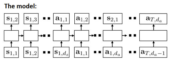
Trajectory Transformer Janner, Li, Levine. Reinforcement Learning as One Big Sequence Modeling Problem. 2021. Model drew with Auto-regressive sequence model Train a joint state-action modelp β ( τ ) = p β ( s 1 , a 2 , … , s T , a T ) p_\beta(\tau) = p_\beta(s_1,a_2, \dots, s_T, a_T) p β ( τ ) = p β ( s 1 , a 2 , … , s T , a T ) Intuitively we want to optimize for a plan for a sequence of actions that has a high probability under the data distribution Use a big expressive model (Transformer)Subscript in the model image just shows the “timestep, dimension” of state and action spaces Diagram is an Auto-regressive sequence model (LSTM) With transformer need a causal maskGPT-style model Because we are regressing on both state and action sequences we can have accurate predictions out to much longer horizons ControlBeam search, but use ∑ t r ( s t , a t ) \sum_t r(s_t,a_t) ∑ t r ( s t , a t ) Given current sequence, sample next tokens from model Store top K K K Other methods like MCTS works as well
This works because
Generating high-probability trajectories avoids OOD states & actions using a really big model works well in offline mode
Which Offline Algorithm to use? If only want to train offlineCQLJust one hyper-param, well understood and widely tested IQLMore flexible (offline + online) Only train offline and finetune onlineAdvantage-weighted actor-critic (AWAC)Widely used an well tested IQLPerforms much better than AWAC! If have a good way to train models in the domainNot always easy to train a good model in a specific domain! COMBOSimilar properties as CQL but benefits from models Trajectory TransformerVery powerful and effective models Extremely computationally expensive to train and evaluate
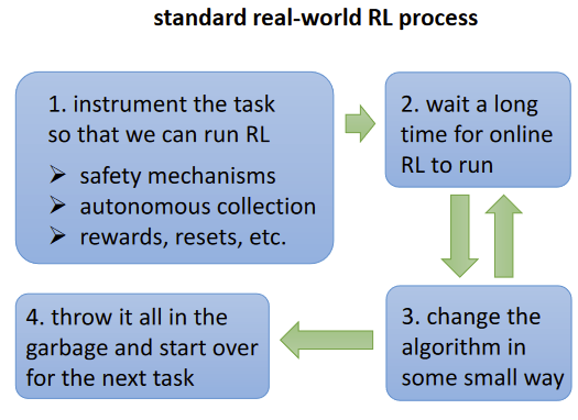
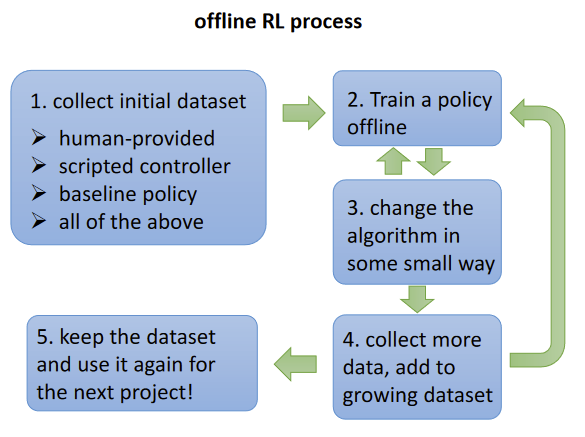
Why offline RL Open Problems An offline RL workflowSupervised learning workflow: train/test split Offline RL workflow: Train offline, evaluate online Starting PointKumar, Singh, Tian, Finn, Levine. A Workflow for Offline Model-Free Robotic Reinforcement Learning. CoRL 2021 Statistical guaranteesBiggest challenge: distributional shift/counterfactuals Can we make any guarantees? Scalable methods, large-scale applicationsData-driven navigation and driving