Policy Gradients ”REINFORCE algorithm” Remember: Direct gradient descent on RL objective
θ ∗ = arg max θ E τ ∼ p θ ( τ ) [ ∑ t r ( s t , a t ) ] undefined J ( θ ) = arg max θ ∑ t = 1 T E ( s t , a t ) ∼ p θ ( s t , a t ) [ r ( s t , a t ) ] \begin{split}
\theta^* &= \argmax_\theta \underbrace{ \mathbb{E}_{\tau \sim p_\theta(\tau)} [\sum_t r(s_t,a_t)] }_{\mathclap{J(\theta)}} \\
&= \argmax_{\theta} \sum_{t=1}^T \mathbb{E}_{(s_t,a_t) \sim p_\theta(s_t,a_t)}[r(s_t,a_t)]
\end{split}
θ ∗ = θ arg max J ( θ ) E τ ∼ p θ ( τ ) [ t ∑ r ( s t , a t )] = θ arg max t = 1 ∑ T E ( s t , a t ) ∼ p θ ( s t , a t ) [ r ( s t , a t )] Note: We don’t know anything about the p ( s 1 ) p(s_1) p ( s 1 ) p ( s i + 1 ∣ a i , s i ) p(s_{i+1}|a_i, s_i) p ( s i + 1 ∣ a i , s i )
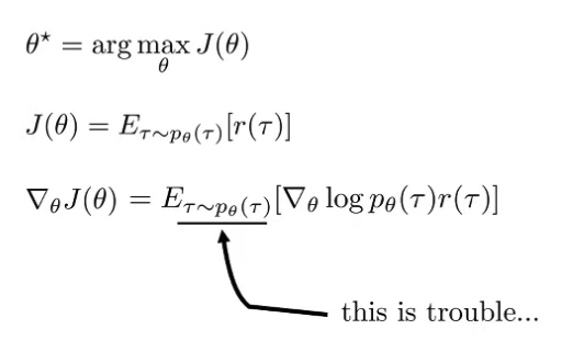
J ( θ ) = E τ ∼ p θ ( τ ) [ ∑ t r ( s t , a t ) undefined denote as r ( τ ) ] = ∫ p θ ( τ ) r ( τ ) d τ ≈ 1 N ∑ i ∑ t r ( s i , t , a i , t undefined Reward of time step t in the i -th sample ) \begin{split}
J(\theta)&=\mathbb{E}_{\tau \sim p_\theta(\tau)}[\underbrace{\sum_t r(s_t,a_t)}_{\mathclap{\text{denote as }r(\tau)}}] \\
&= \int p_\theta(\tau)r(\tau)d\tau \\
&\approx \frac{1}{N} \sum_i \sum_t \underbrace{r(s_{i,t}, a_{i,t}}_{\mathclap{\text{Reward of time step $t$ in the $i$-th sample}}})
\end{split} J ( θ ) = E τ ∼ p θ ( τ ) [ denote as r ( τ ) t ∑ r ( s t , a t ) ] = ∫ p θ ( τ ) r ( τ ) d τ ≈ N 1 i ∑ t ∑ Reward of time step t in the i -th sample r ( s i , t , a i , t ) The larger our sample size N is, the more accurate our estimate will be ∇ θ J ( θ ) = ∫ ∇ θ p θ ( τ ) r ( τ ) d τ \nabla_\theta J(\theta)=\int \nabla_\theta p_\theta(\tau)r(\tau) d\tau ∇ θ J ( θ ) = ∫ ∇ θ p θ ( τ ) r ( τ ) d τ We will use a convenient identity to rewrite this equation so that it can be evaluated without knowing the distribution for p θ ( τ ) p_\theta(\tau) p θ ( τ )
p θ ( τ ) ∇ log p θ ( τ ) = p θ ( τ ) ∇ θ p θ ( τ ) p θ ( τ ) = ∇ θ p θ ( τ ) p_\theta(\tau)\nabla \log p_\theta(\tau) = p_\theta(\tau) \frac{\nabla_\theta p_\theta(\tau)}{p_\theta(\tau)} = \nabla_\theta p_\theta(\tau) p θ ( τ ) ∇ log p θ ( τ ) = p θ ( τ ) p θ ( τ ) ∇ θ p θ ( τ ) = ∇ θ p θ ( τ ) Using this identity, we can rewrite the equation
∇ θ J ( θ ) = ∫ ∇ θ p θ ( τ ) r ( τ ) d τ = ∫ p θ ( τ ) ∇ θ log p θ ( τ ) r ( τ ) d τ \begin{split}
\nabla_\theta J(\theta)
&= \int \nabla_\theta p_\theta(\tau)r(\tau)d\tau \\
&= \int p_\theta(\tau)\nabla_\theta \log p_\theta(\tau)r(\tau)d\tau
\end{split} ∇ θ J ( θ ) = ∫ ∇ θ p θ ( τ ) r ( τ ) d τ = ∫ p θ ( τ ) ∇ θ log p θ ( τ ) r ( τ ) d τ Note:
p θ ( s 1 , a 1 , … , s T , a T ) = p ( s 1 ) ∏ t = 1 T π θ ( a t ∣ s t ) p ( s t + 1 ∣ s t , a t ) log p θ ( s 1 , a 1 , … , s T , a T ) = log p ( s 1 ) + ∑ t = 1 T log π θ ( a t ∣ s t ) + log p ( s t + 1 ∣ s t , a t ) p_\theta(s_1,a_1,\dots,s_T,a_T)=p(s_1)\prod_{t=1}^T \pi_\theta(a_t|s_t) p(s_{t+1}|s_t, a_t) \\
\log p_\theta(s_1,a_1,\dots,s_T,a_T)=\log p(s_1)+ \sum_{t=1}^T \log \pi_\theta(a_t|s_t) + \log p(s_{t+1}|s_t, a_t) p θ ( s 1 , a 1 , … , s T , a T ) = p ( s 1 ) t = 1 ∏ T π θ ( a t ∣ s t ) p ( s t + 1 ∣ s t , a t ) log p θ ( s 1 , a 1 , … , s T , a T ) = log p ( s 1 ) + t = 1 ∑ T log π θ ( a t ∣ s t ) + log p ( s t + 1 ∣ s t , a t ) So if we consider the ∇ θ J ( θ ) \nabla_\theta J(\theta) ∇ θ J ( θ ) ∇ θ log p θ ( τ ) \nabla_\theta \log p_\theta(\tau) ∇ θ log p θ ( τ )
∇ θ log p θ ( τ ) = ∇ θ [ log p ( s 1 ) + ∑ t = 1 T log π θ ( a t ∣ s t ) + log p ( s t + 1 ∣ s t , a t ) ] = ∇ θ ∑ t = 1 T log π θ ( a t ∣ s t ) \begin{split}
\nabla_\theta \log p_\theta(\tau) &= \nabla_\theta[\log p(s_1) + \sum_{t=1}^T \log \pi_\theta(a_t|s_t)+\log p(s_{t+1}|s_t,a_t)] \\
&= \nabla_\theta \sum_{t=1}^T \log \pi_\theta(a_t|s_t)
\end{split} ∇ θ log p θ ( τ ) = ∇ θ [ log p ( s 1 ) + t = 1 ∑ T log π θ ( a t ∣ s t ) + log p ( s t + 1 ∣ s t , a t )] = ∇ θ t = 1 ∑ T log π θ ( a t ∣ s t ) So therefore
∇ θ J ( θ ) = E τ ∼ p θ ( τ ) [ ( ∑ t = 1 T ∇ θ log π θ ( a t ∣ s t ) ) ( ∑ t = 1 T r ( s t , a t ) ) ] ≈ 1 N ∑ i = 1 N ( ∑ t = 1 T ∇ θ log π θ ( a i , t ∣ s i , t ) ( ∑ t = 1 T r ( s i , t , a i , t ) ) \begin{split}
\nabla_\theta J(\theta)&=\mathbb{E}_{\tau \sim p_\theta(\tau)}[(\sum_{t=1}^T\nabla_\theta \log \pi_\theta(a_t|s_t))(\sum_{t=1}^Tr(s_t,a_t))] \\
&\approx \frac{1}{N}\sum_{i=1}^N(\sum_{t=1}^T \nabla_\theta \log \pi_\theta(a_{i,t}|s_{i,t})(\sum_{t=1}^T r(s_{i,t},a_{i,t}))
\end{split} ∇ θ J ( θ ) = E τ ∼ p θ ( τ ) [( t = 1 ∑ T ∇ θ log π θ ( a t ∣ s t )) ( t = 1 ∑ T r ( s t , a t ))] ≈ N 1 i = 1 ∑ N ( t = 1 ∑ T ∇ θ log π θ ( a i , t ∣ s i , t ) ( t = 1 ∑ T r ( s i , t , a i , t )) Improve by
θ ← θ + α ∇ θ J ( θ ) \theta \leftarrow \theta + \alpha\nabla_\theta J(\theta) θ ← θ + α ∇ θ J ( θ )
”REINFORCE algorithm” on continuous space
e.g. We can represent p θ ( a t ∣ s t ) p_\theta(a_t|s_t) p θ ( a t ∣ s t ) N ( f neural network ( s t ) ; Σ ) N(f_{\text{neural network}}(s_t);\Sigma) N ( f neural network ( s t ) ; Σ )
∇ θ log π θ ( a t ∣ s t ) = − 1 2 Σ − 1 ( f ( s t ) − a t ) d f d θ \nabla_{\theta} \log \pi_\theta(a_t|s_t)=-\frac{1}{2}\Sigma^{-1}(f(s_t)-a_t)\frac{df}{d\theta} ∇ θ log π θ ( a t ∣ s t ) = − 2 1 Σ − 1 ( f ( s t ) − a t ) d θ df
Sample { τ i } \{\tau^i\} { τ i } π θ ( a t ∣ s t ) \pi_\theta(a_t|s_t) π θ ( a t ∣ s t ) ∇ θ J ( θ ) ≈ ∑ i ( ∑ t ∇ θ log π θ ( a t i ∣ s t i ) ) ( ∑ t r ( s t i , a t i ) ) \nabla_\theta J(\theta) \approx \sum_i(\sum_t \nabla_\theta \log \pi_\theta(a_t^i|s_t^i))(\sum_t r(s_t^i, a_t^i)) ∇ θ J ( θ ) ≈ ∑ i ( ∑ t ∇ θ log π θ ( a t i ∣ s t i )) ( ∑ t r ( s t i , a t i )) θ ← θ + α ∇ θ J ( θ ) \theta \leftarrow \theta + \alpha \nabla_\theta J(\theta) θ ← θ + α ∇ θ J ( θ )
Partial Observability ∇ θ J ( θ ) ≈ 1 N ∑ i = 1 N ( ∑ t = 1 N ∇ θ log π θ ( a i , t ∣ o i , t ) ) ( ∑ t = 1 T r ( s i , t , a i , t ) ) \nabla_\theta J(\theta) \approx
\frac{1}{N}\sum_{i=1}^N (\sum_{t=1}^N \nabla_\theta \log \pi_\theta (a_{i,t}|o_{i,t}))(\sum_{t=1}^T r(s_{i,t},a_{i,t})) ∇ θ J ( θ ) ≈ N 1 i = 1 ∑ N ( t = 1 ∑ N ∇ θ log π θ ( a i , t ∣ o i , t )) ( t = 1 ∑ T r ( s i , t , a i , t )) 🔥
Markov property is not actually used so we can just use
o i , t o_{i,t} o i , t in place of
s i , t s_{i,t} s i , t
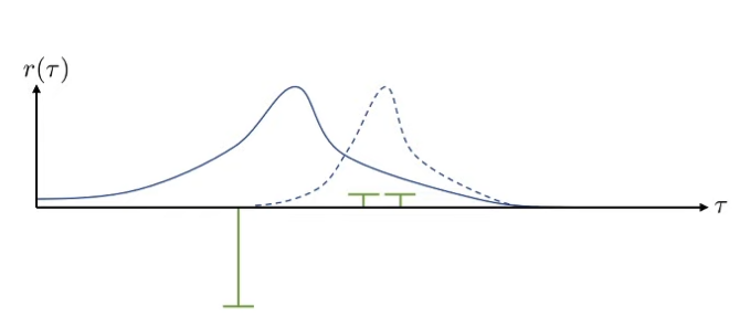
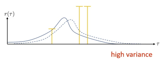
What’s wrong? Blue graph corresponds to PDF of reward, green bars represent samples of rewards, and dashed blue graph corresponds to fitted policy distribution What if reward is shifted up (adding a constant) (while everything maintains the same)? We see huge differences in fitted policy distributions ⇒ we have a high variance problem
How we can modify policy gradient to reduce variance? 🔥
Causality: policy at time
t ’ t’ t ’ cannot affect reward at time
t t t if
t < t ’ t < t’ t < t ’ ∇ θ J ( θ ) ≈ 1 N ∑ i = 1 N ∑ t = 1 T ∇ θ log π θ ( a i , t ∣ s i , t ) ( ∑ t ′ = 1 T r ( s i , t ′ , a i , t ′ ) ) \nabla_\theta J(\theta) \approx \frac{1}{N}\sum_{i=1}^N\sum_{t=1}^T\nabla_\theta\log\pi_\theta(a_{i,t}|s_{i,t})(\sum_{t'=1}^T r(s_{i,t'},a_{i,t'})) ∇ θ J ( θ ) ≈ N 1 i = 1 ∑ N t = 1 ∑ T ∇ θ log π θ ( a i , t ∣ s i , t ) ( t ′ = 1 ∑ T r ( s i , t ′ , a i , t ′ )) We want to show that the expectation of the previous rewards would converge to 0 so we can rewrite the summation. Note that removing those terms in finite time would change the estimator but it is still unbiased.
∇ θ J ( θ ) ≈ 1 N ∑ i = 1 N ∑ t = 1 T ∇ θ log π θ ( a i , t ∣ s i , t ) ( ∑ t ′ = t T r ( s i , t ′ , a i , t ′ ) ) undefined reward to go Q ^ i , t \nabla_\theta J(\theta) \approx \frac{1}{N}\sum_{i=1}^N\sum_{t=1}^T\nabla_\theta\log\pi_\theta(a_{i,t}|s_{i,t})\underbrace{(\sum_{t'=t}^T r(s_{i,t'},a_{i,t'}))}_{\mathclap{\text{reward to go $\hat{Q}_{i,t}$}}} ∇ θ J ( θ ) ≈ N 1 i = 1 ∑ N t = 1 ∑ T ∇ θ log π θ ( a i , t ∣ s i , t ) reward to go Q ^ i , t ( t ′ = t ∑ T r ( s i , t ′ , a i , t ′ )) We have removed some items from the sum therefore the variance is lower.
With discount factors ∇ θ J ( θ ) ≈ 1 N ∑ i = 1 N ∑ t = 1 T ∇ θ log π θ ( a i , t ∣ s i , t ) ( ∑ t ′ = t T γ t ′ − t r ( s i , t ′ , a i , t ) ) \nabla_\theta J(\theta) \approx \frac{1}{N} \sum_{i=1}^N \sum_{t=1}^T \nabla _\theta \log \pi_\theta (a_{i,t}|s_{i,t}) (\sum_{t' = t}^T \gamma^{t' -t} r(s_{i,t'},a_{i,t})) ∇ θ J ( θ ) ≈ N 1 i = 1 ∑ N t = 1 ∑ T ∇ θ log π θ ( a i , t ∣ s i , t ) ( t ′ = t ∑ T γ t ′ − t r ( s i , t ′ , a i , t )) The power on the γ \gamma γ t ’ − t t’ - t t ’ − t
If we let the power be t ’ − 1 t’ - 1 t ’ − 1 t − 1 t-1 t − 1 t = 0 t=0 t = 0 t → ∞ t \rightarrow \infin t → ∞ t t t
Baselines We want policy gradients to optimize reward actions that are above average and penalize reward actions that are below average.
∇ θ J ( θ ) ≈ 1 N ∑ i = 1 N ∇ θ log p θ ( τ ) [ r ( τ ) − b ] \begin{split}
\nabla_\theta J(\theta) &\approx \frac{1}{N} \sum_{i=1}^N
\nabla_\theta \log p_\theta (\tau)[r(\tau)-b]
\end{split} ∇ θ J ( θ ) ≈ N 1 i = 1 ∑ N ∇ θ log p θ ( τ ) [ r ( τ ) − b ] Without baseline (b = 0), but with baseline, set b as
b = 1 N ∑ i = 1 N r ( τ ) b = \frac{1}{N}\sum_{i=1}^Nr(\tau) b = N 1 i = 1 ∑ N r ( τ ) Changing b will keep the esitimator unbiased but will change the variance!
E [ ∇ θ log p θ ( τ ) b ] = ∫ p θ ( τ ) ∇ θ log p θ ( τ ) b d τ = ∫ ∇ θ p θ ( τ ) b d τ = b ∇ θ ∫ p θ ( τ ) d τ = b ∇ θ 1 = 0 \begin{split}
\mathbb{E}[\nabla_\theta \log p_\theta(\tau)b] &= \int p_\theta(\tau)\nabla_\theta \log p_\theta(\tau) b d\tau \\
&= \int \nabla_\theta p_\theta(\tau)b d\tau \\
&= b \nabla_\theta \int p_\theta(\tau) d\tau \\
&=b\nabla_\theta1 = 0
\end{split} E [ ∇ θ log p θ ( τ ) b ] = ∫ p θ ( τ ) ∇ θ log p θ ( τ ) b d τ = ∫ ∇ θ p θ ( τ ) b d τ = b ∇ θ ∫ p θ ( τ ) d τ = b ∇ θ 1 = 0 Average reward is not the best baseline, but it’s pretty good!
Let’s first write down variance
V a r = E τ ∼ p θ ( τ ) [ ( ∇ θ log p θ ( τ ) ( r ( τ ) − b ) ) 2 ] − E τ ∼ p θ ( τ ) [ ∇ θ log p θ ( τ ) ( r ( τ ) − b ) ] 2 \begin{split}
Var &= \mathbb{E}_{\tau \sim p_\theta(\tau)}[(\nabla_\theta \log p_\theta(\tau)(r(\tau)-b))^2]-\mathbb{E}_{\tau \sim p_\theta(\tau)}[\nabla_\theta\log p_\theta (\tau)(r(\tau)-b)]^2 \\
\end{split} Va r = E τ ∼ p θ ( τ ) [( ∇ θ log p θ ( τ ) ( r ( τ ) − b ) ) 2 ] − E τ ∼ p θ ( τ ) [ ∇ θ log p θ ( τ ) ( r ( τ ) − b ) ] 2 d V a r d b = d d b E [ g ( τ ) 2 ( r ( τ ) − b ) 2 ] , g ( τ ) = gradient ( log ( τ ) ) = d d b ( E [ g ( τ ) 2 r ( τ ) 2 ] − 2 E [ g ( τ ) 2 r ( τ ) b ] + b 2 E [ g ( τ ) 2 ] ) = − 2 E [ g ( τ ) 2 r ( τ ) ] + 2 b E [ g ( τ ) 2 ] = 0 \begin{split}
\frac{dVar}{db} &=\frac{d}{db}\mathbb{E}[g(\tau)^2(r(\tau)-b)^2], g(\tau)=\text{gradient$(\log(\tau))$} \\
&=\frac{d}{db}(\mathbb{E}[g(\tau)^2r(\tau)^2]-2\mathbb{E}[g(\tau)^2r(\tau)b]+b^2\mathbb{E}[g(\tau)^2]) \\
&= -2\mathbb{E}[g(\tau)^2r(\tau)]+2b\mathbb{E}[g(\tau)^2]=0 \\
\end{split} d b d Va r = d b d E [ g ( τ ) 2 ( r ( τ ) − b ) 2 ] , g ( τ ) = gradient ( log ( τ )) = d b d ( E [ g ( τ ) 2 r ( τ ) 2 ] − 2 E [ g ( τ ) 2 r ( τ ) b ] + b 2 E [ g ( τ ) 2 ]) = − 2 E [ g ( τ ) 2 r ( τ )] + 2 b E [ g ( τ ) 2 ] = 0 So optimal value of b
b = E [ g ( τ ) 2 r ( τ ) ] E [ g ( τ ) 2 ] b = \frac{\mathbb{E}[g(\tau)^2r(\tau)]}{\mathbb{E}[g(\tau)^2]} b = E [ g ( τ ) 2 ] E [ g ( τ ) 2 r ( τ )] Intuition: Different baseline for every entry in the gradient, the baseline for every parameter value is the expected value of the reward weighted by the magnitude of the gradient for the parameter value
Off-policy setting Policy gradient is defined to be on-policy
The expectatio causes us to need to update samples every time we have updated the policy, but problem is Neural Nets only change a bit with each gradient step .
So we can modify the policy a bit
Instead of having samples from p θ ( τ ) p_\theta(\tau) p θ ( τ ) p ˉ ( τ ) \bar{p}(\tau) p ˉ ( τ )
We can use importance sampling to accomodate this case
E x ∼ p ( x ) [ f ( x ) ] = ∫ P p ( x ) f ( x ) d x = ∫ P q ( x ) P q ( x ) P p ( x ) f ( x ) d x = ∫ P q ( x ) P p ( x ) P q ( x ) f ( x ) d x \begin{split}
\mathbb{E}_{x \sim p(x)}[f(x)] &= \int \mathbb{P}_p(x)f(x)dx \\
&=\int \frac{\mathbb{P}_q (x)}{\mathbb{P}_q (x)} \mathbb{P}_p (x) f(x) dx \\
&=\int \mathbb{P}_q(x) \frac{\mathbb{P}_p(x)}{\mathbb{P}_q(x)}f(x)dx
\end{split} E x ∼ p ( x ) [ f ( x )] = ∫ P p ( x ) f ( x ) d x = ∫ P q ( x ) P q ( x ) P p ( x ) f ( x ) d x = ∫ P q ( x ) P q ( x ) P p ( x ) f ( x ) d x Due to this expectation, we see that our objective becomes this
J ( θ ) = E τ ∼ p ˉ ( τ ) [ p θ ( τ ) p ˉ ( τ ) r ( τ ) ] J(\theta)=\mathbb{E}_{\tau \sim \bar{p}(\tau)}[\frac{p_\theta(\tau)}{\bar{p}(\tau)}r(\tau)] J ( θ ) = E τ ∼ p ˉ ( τ ) [ p ˉ ( τ ) p θ ( τ ) r ( τ )] Where
p θ ( τ ) = p ( s 1 ) ∏ t = 1 T π θ ( a t ∣ s t ) p ( s t + 1 ∣ s t , a t ) p_\theta(\tau)=p(s_1)\prod_{t=1}^T \pi_\theta(a_t|s_t)p(s_{t+1}|s_t,a_t) p θ ( τ ) = p ( s 1 ) t = 1 ∏ T π θ ( a t ∣ s t ) p ( s t + 1 ∣ s t , a t ) Therefore,
p θ ( τ ) p ˉ ( τ ) = p ( s 1 ) ∏ t = 1 T π θ ( a t ∣ s t ) p ( s t + 1 ∣ s t , a t ) p ( s 1 ) ∏ t = 1 T π ˉ θ ( a t ∣ s t ) p ( s t + 1 ∣ s t , a t ) = ∏ t = 1 T π θ ( a t ∣ s t ) ∏ t = 1 T π ˉ θ ( a t ∣ s t ) \begin{split}
\frac{p_\theta(\tau)}{\bar{p}(\tau)} &= \frac{p(s_1)\prod_{t=1}^T \pi_\theta(a_t|s_t)p(s_{t+1}|s_t,a_t)}{p(s_1)\prod_{t=1}^T \bar{\pi}_\theta(a_t|s_t)p(s_{t+1}|s_t,a_t)} \\
&=\frac{\prod_{t=1}^T \pi_\theta(a_t|s_t)}{\prod_{t=1}^T \bar\pi_\theta(a_t|s_t)}
\end{split} p ˉ ( τ ) p θ ( τ ) = p ( s 1 ) ∏ t = 1 T π ˉ θ ( a t ∣ s t ) p ( s t + 1 ∣ s t , a t ) p ( s 1 ) ∏ t = 1 T π θ ( a t ∣ s t ) p ( s t + 1 ∣ s t , a t ) = ∏ t = 1 T π ˉ θ ( a t ∣ s t ) ∏ t = 1 T π θ ( a t ∣ s t ) So… we can estimate the value of some new parameters θ ′ \theta ' θ ′
J ( θ ′ ) = E τ ∼ p θ ( τ ) [ p θ ′ ( τ ) p θ ( τ ) r ( τ ) ] J(\theta')=\mathbb{E}_{\tau \sim p_{\theta}(\tau)}[\frac{p_{\theta'}(\tau)}{p_\theta(\tau)} r(\tau)] J ( θ ′ ) = E τ ∼ p θ ( τ ) [ p θ ( τ ) p θ ′ ( τ ) r ( τ )] ∇ θ ′ J ( θ ′ ) = E τ ∼ p θ ( τ ) [ ∇ θ ′ p θ ′ ( τ ) p θ ( τ ) r ( τ ) ] = E τ ∼ p θ ( τ ) [ p θ ′ ( τ ) p θ ( τ ) ∇ θ ′ log p θ ′ ( τ ) r ( τ ) ] = E τ ∼ p θ ( τ ) [ ( ∏ t = 1 T π θ ′ ( a t ∣ s t ) π θ ( a t ∣ s t ) ) ( ∑ t = 1 T ∇ θ ′ log π θ ′ ( a t ∣ s t ) ) ( ∑ t = 1 T r ( s t , a t ) ) ] \begin{split}
\nabla_{\theta '} J(\theta ') &= \mathbb{E}_{\tau \sim p_\theta(\tau)} [\frac{\nabla_{\theta '} p_{\theta '}(\tau)}{p_\theta(\tau)}r(\tau)] \\
&=\mathbb{E}_{\tau \sim p_\theta(\tau)} [\frac{p_{\theta '}(\tau)}{p_\theta(\tau)}\nabla_{\theta '} \log p_{\theta '} (\tau) r(\tau)] \\
&=\mathbb{E}_{\tau \sim p_\theta(\tau)}[(\prod_{t=1}^T\frac{\pi_{\theta '}(a_t|s_t)}{\pi_\theta(a_t|s_t)})(\sum_{t=1}^T \nabla_{\theta '} \log \pi_{\theta '}(a_t|s_t))(\sum_{t=1}^T r(s_t,a_t))]
\end{split} ∇ θ ′ J ( θ ′ ) = E τ ∼ p θ ( τ ) [ p θ ( τ ) ∇ θ ′ p θ ′ ( τ ) r ( τ )] = E τ ∼ p θ ( τ ) [ p θ ( τ ) p θ ′ ( τ ) ∇ θ ′ log p θ ′ ( τ ) r ( τ )] = E τ ∼ p θ ( τ ) [( t = 1 ∏ T π θ ( a t ∣ s t ) π θ ′ ( a t ∣ s t ) ) ( t = 1 ∑ T ∇ θ ′ log π θ ′ ( a t ∣ s t )) ( t = 1 ∑ T r ( s t , a t ))] We can consider causality(the fact that current action does not affect past rewards) and
∇ θ ′ J ( θ ′ ) = E τ ∼ p θ ( τ ) [ ∑ t = 1 T ∇ θ ′ log π θ ′ ( a t ∣ s t ) ( ∏ t ′ = 1 t π θ ′ ( a t ′ ∣ s t ′ ) π θ ( a t ′ ∣ s t ′ ) ) ( ∑ t ′ = t T r ( s t ′ , a t ′ ) ( ∏ t ′ ′ = t t ′ π θ ′ ( a t ′ ′ ∣ s t ′ ′ ) π θ ( a t ′ ′ ∣ s t ′ ′ ) ) ) ] \begin{split}
\nabla_{\theta '} J(\theta ')
&=\mathbb{E}_{\tau \sim p_\theta(\tau)}[\sum_{t=1}^T \nabla_{\theta '} \log \pi_{\theta '}(a_t|s_t)(\prod_{t'=1}^t \frac{\pi_{\theta '} (a_{t'}|s_{t'})}{\pi_\theta(a_{t '}|s_{t '})})(\sum_{t' = t}^Tr(s_{t'},a_{t'})(\prod_{t''=t}^{t'}\frac{\pi_{\theta '}(a_{t ''}|s_{t ''})}{\pi_\theta(a_{t ''} | s_{t ''})}))]
\end{split} ∇ θ ′ J ( θ ′ ) = E τ ∼ p θ ( τ ) [ t = 1 ∑ T ∇ θ ′ log π θ ′ ( a t ∣ s t ) ( t ′ = 1 ∏ t π θ ( a t ′ ∣ s t ′ ) π θ ′ ( a t ′ ∣ s t ′ ) ) ( t ′ = t ∑ T r ( s t ′ , a t ′ ) ( t ′′ = t ∏ t ′ π θ ( a t ′′ ∣ s t ′′ ) π θ ′ ( a t ′′ ∣ s t ′′ ) ))] Some important terms in this equation:
∏ t ’ = 1 t π θ ‘ ( a t ‘ ∣ s t ’ ) π θ ( a t ‘ ∣ s t ’ ) \prod_{t’=1}^t \frac{\pi_{\theta ‘}(a_{t ‘} | s_{t ’})}{\pi_{\theta}(a_{t ‘} | s_{t ’})} ∏ t ’ = 1 t π θ ( a t ‘ ∣ s t ’ ) π θ ‘ ( a t ‘ ∣ s t ’ ) exponential in T T T
∏ t ′ ′ = t t ′ π θ ′ ( a t ′ ′ ∣ s t ′ ′ ) π θ ( a t ′ ′ ∣ s t ′ ′ ) \prod_{t''=t}^{t'}\frac{\pi_{\theta '}(a_{t ''}|s_{t ''})}{\pi_\theta(a_{t ''} | s_{t ''})} ∏ t ′′ = t t ′ π θ ( a t ′′ ∣ s t ′′ ) π θ ′ ( a t ′′ ∣ s t ′′ )
Since the first term is exponential, we can try to write the objetive a bit differently
On-policy policy gradient
∇ θ J ( θ ) ≈ 1 N ∑ i = 1 N ∑ t = 1 T ∇ θ log π θ ( a i , t ∣ s i , t ) Q ^ i , t \nabla_\theta J(\theta) \approx \frac{1}{N} \sum_{i=1}^N \sum_{t=1}^T \nabla_\theta \log \pi_\theta(a_{i,t}|s_{i,t}) \hat{Q}_{i,t} ∇ θ J ( θ ) ≈ N 1 i = 1 ∑ N t = 1 ∑ T ∇ θ log π θ ( a i , t ∣ s i , t ) Q ^ i , t Off-policy policy gradient
∇ θ ′ J ( θ ′ ) ≈ 1 N ∑ i = 1 N ∑ t = 1 T π θ ′ ( s i , t , a i , t ) π θ ( s i , t , a i , t ) ∇ θ ′ log π θ ′ ( a i , t ∣ s i , t ) Q ^ i , t = 1 N ∑ i = 1 N ∑ t = 1 T π θ ′ ( s i , t ) π θ ( s i , t ) undefined Can we ignore this part? π θ ′ ( a i , t ∣ s i , t ) π θ ( a i , t ∣ s i , t ) ∇ θ ′ log π θ ′ ( a i , t ∣ s i , t ) Q ^ i , t \begin{split}
\nabla_{\theta '} J(\theta ') &\approx \frac{1}{N}\sum_{i=1}^N\sum_{t=1}^T \frac{\pi_{\theta '} (s_{i,t}, a_{i,t})}{\pi_\theta(s_{i,t},a_{i,t})} \nabla_{\theta '} \log \pi_{\theta '}(a_{i,t}|s_{i,t}) \hat{Q}_{i,t} \\
&\quad = \frac{1}{N}\sum_{i=1}^N \sum_{t=1}^T
\underbrace{\frac{\pi_{\theta '}(s_{i,t})}{\pi_\theta(s_{i,t})}}_{\mathclap{\text{Can we ignore this part?}}} \frac{\pi_{\theta '}(a_{i,t}|s_{i,t})}{\pi_\theta(a_{i,t}|s_{i,t})} \nabla_{\theta '} \log \pi_{\theta '}(a_{i,t}|s_{i,t}) \hat{Q}_{i,t}
\end{split} ∇ θ ′ J ( θ ′ ) ≈ N 1 i = 1 ∑ N t = 1 ∑ T π θ ( s i , t , a i , t ) π θ ′ ( s i , t , a i , t ) ∇ θ ′ log π θ ′ ( a i , t ∣ s i , t ) Q ^ i , t = N 1 i = 1 ∑ N t = 1 ∑ T Can we ignore this part? π θ ( s i , t ) π θ ′ ( s i , t ) π θ ( a i , t ∣ s i , t ) π θ ′ ( a i , t ∣ s i , t ) ∇ θ ′ log π θ ′ ( a i , t ∣ s i , t ) Q ^ i , t This does not necessarily give the optimal policy, but its a reasonable approximation.
Policy Gradient with Automatic Differentiation We don’t want to be inefficient at computing gradients ⇒ use backprop trick
So why don’t we start from the MLE approach to Policy Gradients?
∇ θ J M L ≈ 1 N ∑ i = 1 N ∑ t = 1 T ∇ θ log π θ ( a i , t ∣ s i , t ) \nabla_\theta J_{ML} \approx \frac{1}{N} \sum_{i=1}^N \sum_{t=1}^T \nabla_\theta \log \pi_\theta (a_{i,t}|s_{i,t}) ∇ θ J M L ≈ N 1 i = 1 ∑ N t = 1 ∑ T ∇ θ log π θ ( a i , t ∣ s i , t ) To start doing backprop, let’s define the objective function first.
J M L ( θ ) ≈ 1 N ∑ i = 1 N ∑ t = 1 T log π θ ( a i , t ∣ s i , t ) J_{ML}(\theta) \approx \frac{1}{N}\sum_{i=1}^N \sum_{t=1}^T \log \pi_\theta (a_{i,t}|s_{i,t}) J M L ( θ ) ≈ N 1 i = 1 ∑ N t = 1 ∑ T log π θ ( a i , t ∣ s i , t ) So we will define our “pseudo-loss” approximation as weighted maximum likelihood
J ~ ( θ ) ≈ 1 N ∑ i = 1 N ∑ t = 1 T log π θ ( a i , t ∣ s i , t ) Q ^ i , t \tilde{J}(\theta) \approx \frac{1}{N}\sum_{i=1}^N \sum_{t=1}^T \log \pi_\theta (a_{i,t}|s_{i,t}) \hat{Q}_{i,t} J ~ ( θ ) ≈ N 1 i = 1 ∑ N t = 1 ∑ T log π θ ( a i , t ∣ s i , t ) Q ^ i , t A few reminders about tuning hyper-parameters Gradients has very high varianceIsn’t the same as supervised learning Consider using much larger batches Tweaking learning rates is VERY hardAdaptive step size rules like ADAM can be OK-ish
Covariant/natural policy gradient 🤔
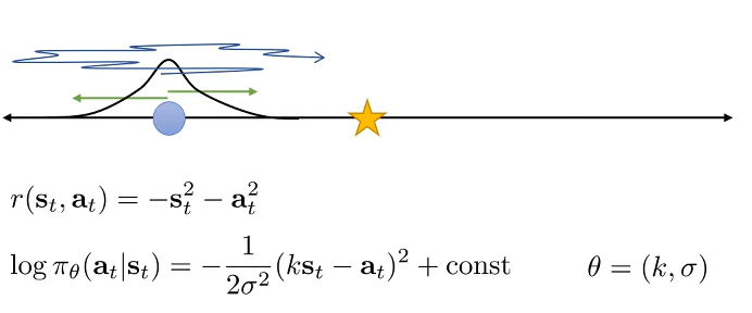
One thing about one dimension state and action spaces are that you can visualize the policy distribution easily one a 2d plane
θ ← θ + α ∇ θ J ( θ ) \theta \leftarrow \theta + \alpha \nabla_\theta J(\theta) θ ← θ + α ∇ θ J ( θ ) We can view the first order gradient descent as follows
θ ′ ← arg max θ ′ ( θ ′ − θ ) ⊤ ∇ θ J ( θ ) s.t. ∣ ∣ θ ′ − θ ∣ ∣ 2 ≤ ϵ \theta ' \leftarrow \argmax_{\theta '} (\theta ' - \theta)^{\top}\nabla_{\theta}J(\theta) \\
\text{s.t. } ||\theta ' - \theta||^2 \le \epsilon θ ′ ← θ ′ arg max ( θ ′ − θ ) ⊤ ∇ θ J ( θ ) s.t. ∣∣ θ ′ − θ ∣ ∣ 2 ≤ ϵ Thank about ϵ \epsilon ϵ
We can instead put constraint on the distribution of the policy
θ ′ ← arg max θ ′ ( θ ′ − θ ) ⊤ ∇ θ J ( θ ) s.t. D ( π θ ′ , π θ ) ≤ ϵ \theta ' \leftarrow \argmax_{\theta '} (\theta ' - \theta)^{\top}\nabla_{\theta}J(\theta) \\
\text{s.t. } D(\pi_{\theta '}, \pi_\theta) \le \epsilon θ ′ ← θ ′ arg max ( θ ′ − θ ) ⊤ ∇ θ J ( θ ) s.t. D ( π θ ′ , π θ ) ≤ ϵ Where D ( ⋅ , ⋅ ) D(\cdot, \cdot) D ( ⋅ , ⋅ )
So we want to choose some parameterization-independent divergence measure
Usually KL-divergence
D K L ( π θ ′ ∣ ∣ π θ ) = E π θ ′ [ log π θ − log π θ ′ ] D_{KL}(\pi_{\theta '}||\pi_\theta) = \mathbb{E}_{\pi_{\theta '}}[\log \pi_\theta - \log \pi_{\theta '}] D K L ( π θ ′ ∣∣ π θ ) = E π θ ′ [ log π θ − log π θ ′ ] A but hard to plug into our gradient descent ⇒ we will approximate this distance using 2nd order Taylor expansion around the current parameter value θ \theta θ
Advanced Policy Gradients Why does policy gradient work? Estimate A ^ π ( s t , a t ) \hat{A}^\pi (s_t,a_t) A ^ π ( s t , a t ) π \pi π Use A ^ π ( s t , a t ) \hat{A}^\pi(s_t,a_t) A ^ π ( s t , a t ) π ′ \pi ' π ′
We are going back and forth between (1) and (2)
Looks familiar to policy iteration algorithm!
Nice thing about policy gradients:
If advantage estimator is perfect, we are just moving closer to the “optimal” policy for the advantage estimator not jumping to the optimal
But how do we formalize this?
If we set the loss function of policy gradient as
J ( θ ) = E τ ∼ p θ ( τ ) [ ∑ t γ t r ( s t , a t ) ] J(\theta) = \mathbb{E}_{\tau \sim p_\theta(\tau)}[\sum_t \gamma^t r(s_t,a_t)] J ( θ ) = E τ ∼ p θ ( τ ) [ t ∑ γ t r ( s t , a t )] Then we can calculate how much we improved by
J ( θ ′ ) − J ( θ ) = E τ ∼ p θ ′ ( τ ) [ ∑ t γ t A π θ ( s t , a t ) ] J(\theta ') - J(\theta) = \mathbb{E}_{\tau \sim p_{\theta'}(\tau)}[\sum_t \gamma^t A^{\pi_\theta}(s_t,a_t)] J ( θ ′ ) − J ( θ ) = E τ ∼ p θ ′ ( τ ) [ t ∑ γ t A π θ ( s t , a t )] Here we claimed that J ( θ ’ ) − J ( θ ) J(\theta’) - J(\theta) J ( θ ’ ) − J ( θ )
We will prove by:
J ( θ ′ ) − J ( θ ) = J ( θ ′ ) − E s 0 ∼ p ( s 0 ) [ V π θ ( s 0 ) ] = J ( θ ′ ) − E τ ∼ p θ ′ ( τ ) [ V π θ ( s 0 ) ] undefined It’s the same as above because the initial states s 0 are the same = J ( θ ′ ) − E τ ∼ p θ ′ ( τ ) [ ∑ t = 0 ∞ γ t V π θ ( s t ) − ∑ t = 1 ∞ γ t V π θ ( s t ) ] = J ( θ ′ ) + E τ ∼ p θ ′ ( τ ) [ ∑ t = 0 ∞ γ t ( γ V π θ ( s t + 1 ) − V π θ ( s t ) ) ] = E τ ∼ p θ ′ ( τ ) [ ∑ t = 0 ∞ γ t r ( s t , a t ) ] + E τ ∼ p θ ′ ( τ ) [ ∑ t = 0 ∞ γ t ( γ V π θ ( s t + 1 ) − V π θ ( s t ) ) ] = E τ ∼ p θ ′ ( τ ) [ ∑ t = 0 ∞ γ t ( r ( s t , a t ) + γ V π θ ( s t + 1 ) − V π θ ( s t ) ) ] = E τ ∼ p θ ′ ( τ ) [ ∑ t = 0 ∞ γ t A π θ ( s t , a t ) ] \begin{split}
J(\theta')-J(\theta)&=J(\theta')-\mathbb{E}_{s_0 \sim p(s_0)} [V^{\pi_\theta}(s_0)] \\
&= J(\theta') - \underbrace{\mathbb{E}_{\tau \sim p_{\theta '}(\tau)}[V^{\pi_\theta}(s_0)]}_{\mathclap{\text{It's the same as above because the initial states $s_0$ are the same}}} \\
&= J(\theta') - \mathbb{E}_{\tau \sim p_{\theta'}(\tau)}[\sum_{t=0}^\infin \gamma^t V^{\pi_\theta}(s_t) - \sum_{t=1}^\infin \gamma^t V^{\pi_\theta}(s_t)] \\
&= J(\theta') + \mathbb{E}_{\tau \sim p_{\theta'}(\tau)}[\sum_{t=0}^\infin \gamma^t (\gamma V^{\pi_\theta}(s_{t+1}) - V^{\pi_\theta}(s_t))] \\
&= \mathbb{E}_{\tau \sim p_{\theta'}(\tau)}[\sum_{t=0}^\infin \gamma^t r(s_t,a_t)] + \mathbb{E}_{\tau \sim p_{\theta'}(\tau)}[\sum_{t=0}^\infin \gamma^t (\gamma V^{\pi_\theta}(s_{t+1}) - V^{\pi_\theta}(s_t))] \\
&= \mathbb{E}_{\tau \sim p_{\theta'}(\tau)}[\sum_{t=0}^\infin \gamma^t (r(s_t,a_t) + \gamma V^{\pi_\theta}(s_{t+1}) - V^{\pi_\theta}(s_t))] \\
&= \mathbb{E}_{\tau \sim p_{\theta'}(\tau)}[\sum_{t=0}^\infin \gamma^t A^{\pi_\theta}(s_t,a_t)]
\end{split} J ( θ ′ ) − J ( θ ) = J ( θ ′ ) − E s 0 ∼ p ( s 0 ) [ V π θ ( s 0 )] = J ( θ ′ ) − It’s the same as above because the initial states s 0 are the same E τ ∼ p θ ′ ( τ ) [ V π θ ( s 0 )] = J ( θ ′ ) − E τ ∼ p θ ′ ( τ ) [ t = 0 ∑ ∞ γ t V π θ ( s t ) − t = 1 ∑ ∞ γ t V π θ ( s t )] = J ( θ ′ ) + E τ ∼ p θ ′ ( τ ) [ t = 0 ∑ ∞ γ t ( γ V π θ ( s t + 1 ) − V π θ ( s t ))] = E τ ∼ p θ ′ ( τ ) [ t = 0 ∑ ∞ γ t r ( s t , a t )] + E τ ∼ p θ ′ ( τ ) [ t = 0 ∑ ∞ γ t ( γ V π θ ( s t + 1 ) − V π θ ( s t ))] = E τ ∼ p θ ′ ( τ ) [ t = 0 ∑ ∞ γ t ( r ( s t , a t ) + γ V π θ ( s t + 1 ) − V π θ ( s t ))] = E τ ∼ p θ ′ ( τ ) [ t = 0 ∑ ∞ γ t A π θ ( s t , a t )] 🔥
This proof shows that by optimizing
E τ ∼ p θ ’ [ ∑ t γ t A π θ ( s t , a t ) ] \mathbb{E}_{\tau \sim p_{\theta’}}[\sum_t \gamma^t A^{\pi_\theta}(s_t,a_t)] E τ ∼ p θ ’ [ ∑ t γ t A π θ ( s t , a t )] , we are actually improving our policy
But how does this relate to our policy gradient? E τ ∼ p θ ′ ( τ ) [ ∑ t γ t A π θ ( s t , a t ) ] = ∑ t E s t ∼ p θ ′ ( s t ) [ E a t ∼ π θ ′ ( a t ∣ s t ) [ γ t A π θ ( s t , a t ) ] ] = ∑ t E s t ∼ p θ ′ ( s t ) [ E a t ∼ π θ ( a t ∣ s t ) [ π θ ′ ( a t ∣ s t ) π θ ( a t ∣ s t ) undefined importance sampling γ t A π θ ( s t , a t ) ] ] ≈ ∑ t E s t ∼ p θ ( s t ) undefined ignoring distribution mismatch [ E a t ∼ π θ ( a t ∣ s t ) [ π θ ′ ( a t ∣ s t ) π θ ( a t ∣ s t ) γ t A π θ ( s t , a t ) ] ] = A ˉ ( θ ′ ) \begin{split}
\mathbb{E}_{\tau\ \sim p_{\theta'}(\tau)}[\sum_t \gamma^t A^{\pi_\theta}(s_t,a_t)]
&= \sum_t \mathbb{E}_{s_t \sim p_{\theta'}(s_t)} [\mathbb{E}_{a_t \sim \pi_{\theta '}(a_t|s_t)}[\gamma^t A^{\pi_\theta} (s_t,a_t)]] \\
&= \sum_t \mathbb{E}_{s_t \sim p_{\theta'}(s_t)} [\underbrace{\mathbb{E}_{a_t \sim \pi_{\theta}(a_t|s_t)}[\frac{\pi_{\theta '}(a_t|s_t)}{\pi_\theta(a_t|s_t)}}_{\mathclap{\text{importance sampling}}} \gamma^t A^{\pi_\theta} (s_t,a_t)]] \\
&\approx \sum_t \underbrace{\mathbb{E}_{s_t \sim p_{\theta}(s_t)}}_{\mathclap{\text{ignoring distribution mismatch}}} [\mathbb{E}_{a_t \sim \pi_{\theta}(a_t|s_t)}[\frac{\pi_{\theta '}(a_t|s_t)}{\pi_\theta(a_t|s_t)} \gamma^t A^{\pi_\theta} (s_t,a_t)]] \\
&\quad =\bar{A}(\theta')
\end{split} E τ ∼ p θ ′ ( τ ) [ t ∑ γ t A π θ ( s t , a t )] = t ∑ E s t ∼ p θ ′ ( s t ) [ E a t ∼ π θ ′ ( a t ∣ s t ) [ γ t A π θ ( s t , a t )]] = t ∑ E s t ∼ p θ ′ ( s t ) [ importance sampling E a t ∼ π θ ( a t ∣ s t ) [ π θ ( a t ∣ s t ) π θ ′ ( a t ∣ s t ) γ t A π θ ( s t , a t )]] ≈ t ∑ ignoring distribution mismatch E s t ∼ p θ ( s t ) [ E a t ∼ π θ ( a t ∣ s t ) [ π θ ( a t ∣ s t ) π θ ′ ( a t ∣ s t ) γ t A π θ ( s t , a t )]] = A ˉ ( θ ′ ) We want this approximation to be true so that
J ( θ ′ ) − J ( θ ) ≈ A ˉ ( θ ′ ) J(\theta')-J(\theta) \approx \bar{A}(\theta') J ( θ ′ ) − J ( θ ) ≈ A ˉ ( θ ′ ) And then we can use
θ ′ ← arg max θ ′ A ˉ ( θ ) \theta' \leftarrow \argmax_{\theta'} \bar{A}(\theta) θ ′ ← θ ′ arg max A ˉ ( θ ) to optimize our policy
And use A ^ π ( s t , a t ) \hat{A}^\pi(s_t,a_t) A ^ π ( s t , a t ) π ’ \pi’ π ’
But when is this true?
Bounding the distribution change (deterministic) We will show:
🔥
p θ ( s t ) p_\theta(s_t) p θ ( s t ) is close to
p θ ’ ( s t ) p_{\theta’}(s_t) p θ ’ ( s t ) when
π θ \pi_\theta π θ is close to
π θ ’ \pi_\theta’ π θ ’ We will assume that π θ \pi_\theta π θ a t = π θ ( s t ) a_t = \pi_\theta(s_t) a t = π θ ( s t )
We define closeness of policy as:
π θ ’ \pi_{\theta’} π θ ’ π θ \pi_\theta π θ π θ ’ ( a t ≠ π θ ( s t ) ∣ s t ) ≤ ϵ \pi_{\theta’}(a_t \ne \pi_\theta(s_t)|s_t) \le \epsilon π θ ’ ( a t = π θ ( s t ) ∣ s t ) ≤ ϵ p θ ′ ( s t ) = ( 1 − ϵ ) t undefined probability we made no mistakes p θ ( s t ) + ( 1 − ( 1 − ϵ ) t ) p m i s t a k e ( s t ) undefined some other distribution p_{\theta'}(s_t) = \underbrace{(1-\epsilon)^t}_{\mathclap{\text{probability we made no mistakes}}} p_\theta(s_t)+(1-(1-\epsilon)^t)\underbrace{p_{mistake}(s_t)}_{\mathclap{\text{some other distribution}}} p θ ′ ( s t ) = probability we made no mistakes ( 1 − ϵ ) t p θ ( s t ) + ( 1 − ( 1 − ϵ ) t ) some other distribution p mi s t ak e ( s t ) Implies that we can write the total variation divergence as
∣ p θ ′ ( s t ) − p θ ( s t ) ∣ = ( 1 − ( 1 − ϵ ) t ) ∣ p m i s t a k e ( s t ) − p θ ( s t ) ∣ ≤ 2 ( 1 − ( 1 − ϵ ) t ) ≤ 2 ϵ t \begin{split}
|p_{\theta'}(s_t)-p_\theta(s_t)|
&= (1-(1-\epsilon)^t) |p_{mistake}(s_t)-p_\theta(s_t)| \\
&\le 2(1-(1-\epsilon)^t) \\
&\le 2\epsilon t
\end{split} ∣ p θ ′ ( s t ) − p θ ( s t ) ∣ = ( 1 − ( 1 − ϵ ) t ) ∣ p mi s t ak e ( s t ) − p θ ( s t ) ∣ ≤ 2 ( 1 − ( 1 − ϵ ) t ) ≤ 2 ϵ t 👉
Useful Identity
∀ ϵ ∈ [ 0 , 1 ] , ( 1 − ϵ ) t ≥ 1 − ϵ t \forall \epsilon \in [0,1], (1-\epsilon)^t \ge 1 - \epsilon t ∀ ϵ ∈ [ 0 , 1 ] , ( 1 − ϵ ) t ≥ 1 − ϵ t
Bounding the distribution change (arbitrary) Schulman, Levine, Moritz, Jordan, Abbeel, “Trust Region Policy Optimization” We will show:
🔥
p θ ( s t ) p_\theta(s_t) p θ ( s t ) is close to
p θ ’ ( s t ) p_{\theta’}(s_t) p θ ’ ( s t ) when
π θ \pi_\theta π θ is close to
π θ ’ \pi_\theta’ π θ ’ Closeness:
π θ ’ \pi_{\theta’} π θ ’ π θ \pi_\theta π θ ∣ π θ ’ ( a t ∣ s t ) − π θ ( a t ∣ s t ) ∣ ≤ ϵ |\pi_{\theta’}(a_t|s_t) - \pi_\theta(a_t|s_t)| \le \epsilon ∣ π θ ’ ( a t ∣ s t ) − π θ ( a t ∣ s t ) ∣ ≤ ϵ s t s_t s t
Useful Lemma:
If ∣ p X ( x ) − p Y ( y ) ∣ = ϵ |p_X(x) - p_Y(y)| = \epsilon ∣ p X ( x ) − p Y ( y ) ∣ = ϵ p ( x , y ) p(x,y) p ( x , y ) p ( x ) = p X ( x ) p(x) = p_X(x) p ( x ) = p X ( x ) p ( y ) = p Y ( y ) p(y) = p_Y(y) p ( y ) = p Y ( y ) p ( x = y ) = 1 − ϵ p(x=y) = 1 - \epsilon p ( x = y ) = 1 − ϵ
Says:
p X ( x ) p_X(x) p X ( x ) p Y ( y ) p_Y(y) p Y ( y ) ϵ \epsilon ϵ π θ ′ ( a t ∣ s t ) \pi_{\theta'}(a_t|s_t) π θ ′ ( a t ∣ s t ) π θ ( a t ∣ s t ) \pi_{\theta}(a_t|s_t) π θ ( a t ∣ s t ) ϵ \epsilon ϵ
Therefore
∣ p θ ′ ( s t ) − p θ ( s t ) ∣ = ( 1 − ( 1 − ϵ ) t ) ∣ p m i s t a k e ( s t ) − p θ ( s t ) ∣ ≤ 2 ( 1 − ( 1 − ϵ ) t ) ≤ 2 ϵ t \begin{split}
|p_{\theta'}(s_t)-p_{\theta}(s_t)| &= (1-(1-\epsilon)^t)|p_{mistake}(s_t)-p_\theta(s_t)| \\
&\le 2(1-(1-\epsilon)^t) \\
&\le 2 \epsilon t
\end{split} ∣ p θ ′ ( s t ) − p θ ( s t ) ∣ = ( 1 − ( 1 − ϵ ) t ) ∣ p mi s t ak e ( s t ) − p θ ( s t ) ∣ ≤ 2 ( 1 − ( 1 − ϵ ) t ) ≤ 2 ϵ t Bounding the objective value Assume ∣ p θ ’ ( s t ) − p θ ( s t ) ∣ ≤ 2 ϵ t |p_{\theta’}(s_t)-p_{\theta}(s_t)| \le 2\epsilon t ∣ p θ ’ ( s t ) − p θ ( s t ) ∣ ≤ 2 ϵ t
E s t ∼ p θ ′ ( s t ) [ f ( s t ) ] = ∑ s t p θ ′ ( s t ) f ( s t ) ≥ ∑ s t p θ ( s t ) f ( s t ) − ∣ p θ ( s t ) − p θ ′ ( s t ) ∣ max s t f ( s t ) ≥ E p θ ( s t ) [ f ( s t ) ] − 2 ϵ t max s t f ( s t ) \begin{split}
\mathbb{E}_{s_t \sim p_{\theta'}(s_t)}[f(s_t)]
&= \sum_{s_t} p_{\theta'}(s_t)f(s_t) \\
&\ge \sum_{s_t} p_{\theta}(s_t)f(s_t) - |p_{\theta}(s_t)-p_{\theta'}(s_t)|\max_{s_t}f(s_t) \\
&\ge \mathbb{E}_{p_\theta(s_t)}[f(s_t)] - 2\epsilon t \max_{s_t} f(s_t)
\end{split} E s t ∼ p θ ′ ( s t ) [ f ( s t )] = s t ∑ p θ ′ ( s t ) f ( s t ) ≥ s t ∑ p θ ( s t ) f ( s t ) − ∣ p θ ( s t ) − p θ ′ ( s t ) ∣ s t max f ( s t ) ≥ E p θ ( s t ) [ f ( s t )] − 2 ϵ t s t max f ( s t ) For the objective value, we can bound it by
E τ ∼ p θ ′ ( τ ) [ ∑ t γ t A π θ ( s t , a t ) ] = ∑ t E s t ∼ p θ ′ ( s t ) [ E a t ∼ π θ ( a t ∣ s t ) [ π θ ′ ( a t ∣ s t ) π θ ( a t ∣ s t ) undefined importance sampling γ t A π θ ( s t , a t ) ] ] ≥ ∑ t E s t ∼ p θ ( s t ) [ E a t ∼ π θ ( a t ∣ s t ) [ π θ ′ ( a t ∣ s t ) π θ ( a t ∣ s t ) γ t A π θ ( s t , a t ) ] ] − ∑ t 2 ϵ t C \begin{split}
\mathbb{E}_{\tau\ \sim p_{\theta'}(\tau)}[\sum_t \gamma^t A^{\pi_\theta}(s_t,a_t)]
&= \sum_t \mathbb{E}_{s_t \sim p_{\theta'}(s_t)} [\underbrace{\mathbb{E}_{a_t \sim \pi_{\theta}(a_t|s_t)}[\frac{\pi_{\theta '}(a_t|s_t)}{\pi_\theta(a_t|s_t)}}_{\mathclap{\text{importance sampling}}} \gamma^t A^{\pi_\theta} (s_t,a_t)]] \\
& \ge \sum_t \mathbb{E}_{s_t \sim p_{\theta}(s_t)} [\mathbb{E}_{a_t \sim \pi_{\theta}(a_t|s_t)}[\frac{\pi_{\theta '}(a_t|s_t)}{\pi_\theta(a_t|s_t)} \gamma^t A^{\pi_\theta} (s_t,a_t)]] - \sum_{t} 2\epsilon tC \\
\end{split} E τ ∼ p θ ′ ( τ ) [ t ∑ γ t A π θ ( s t , a t )] = t ∑ E s t ∼ p θ ′ ( s t ) [ importance sampling E a t ∼ π θ ( a t ∣ s t ) [ π θ ( a t ∣ s t ) π θ ′ ( a t ∣ s t ) γ t A π θ ( s t , a t )]] ≥ t ∑ E s t ∼ p θ ( s t ) [ E a t ∼ π θ ( a t ∣ s t ) [ π θ ( a t ∣ s t ) π θ ′ ( a t ∣ s t ) γ t A π θ ( s t , a t )]] − t ∑ 2 ϵ tC Where C C C
So:
C ∈ O ( T r m a x ) or O ( r m a x 1 − γ ) undefined infinite time with discount (geometric series) C \in O(Tr_{max}) \text{ or } \underbrace{O(\frac{r_{max}}{1-\gamma})}_{\mathclap{\text{infinite time with discount (geometric series)}}} C ∈ O ( T r ma x ) or infinite time with discount (geometric series) O ( 1 − γ r ma x ) Therefore for small enought ϵ \epsilon ϵ A ˉ π ( θ ′ ) \bar{A}^{\pi}(\theta ') A ˉ π ( θ ′ )
Policy Gradients with Constraints We want to constrain:
∣ π θ ′ ( a t ∣ s t ) − π θ ( a t ∣ s t ) ∣ ≤ ϵ |\pi_{\theta'}(a_t|s_t) - \pi_{\theta}(a_t|s_t)| \le \epsilon ∣ π θ ′ ( a t ∣ s t ) − π θ ( a t ∣ s t ) ∣ ≤ ϵ It which will result in
∣ p θ ′ ( s t ) − p θ ( s t ) ∣ ≤ 2 ϵ t |p_{\theta'}(s_t)-p_\theta(s_t)| \le 2\epsilon t ∣ p θ ′ ( s t ) − p θ ( s t ) ∣ ≤ 2 ϵ t A more convenient bound:
∣ π θ ′ ( a t ∣ s t ) − π θ ( a t ∣ s t ) ∣ ≤ 1 2 D K L ( π θ ′ ( a t ∣ s t ) , π θ ( a t ∣ s t ) ) |\pi_{\theta'}(a_t|s_t) - \pi_{\theta}(a_t|s_t)| \le \sqrt{\frac{1}{2} D_{KL}(\pi_{\theta'}(a_t|s_t),\pi_{\theta}(a_t|s_t))} ∣ π θ ′ ( a t ∣ s t ) − π θ ( a t ∣ s t ) ∣ ≤ 2 1 D K L ( π θ ′ ( a t ∣ s t ) , π θ ( a t ∣ s t )) We see that the KL divergence bounds the state marginal difference
Note:
D K L ( p 1 ( x ) , p 2 ( x ) ) = E x ∼ p 1 ( x ) [ log p 1 ( x ) p 2 ( x ) ] D_{KL}(p_1(x),p_2(x)) = \mathbb{E}_{x \sim p_1(x)} [\log \frac{p_1(x)}{p_2(x)}] D K L ( p 1 ( x ) , p 2 ( x )) = E x ∼ p 1 ( x ) [ log p 2 ( x ) p 1 ( x ) ] 👉
KL Divergence has very convenient properties that make it much easier to approximate
So contraining our objective, we have:
θ ′ ← arg max θ ′ ∑ t E s t ∼ p θ ( s t ) [ E a t ∼ π θ ( a t ∣ s t ) [ π θ ′ ( a t ∣ s t ) π θ ( a t ∣ s t ) γ t A π θ ( s t , a t ) ] ] s.t. D K L ( π θ ′ ( a t ∣ s t ) , π θ ( a t ∣ s t ) ) ≤ ϵ \theta' \leftarrow \argmax_{\theta'} \sum_t \mathbb{E}_{s_t \sim p_{\theta}(s_t)}[\mathbb{E}_{a_t \sim \pi_\theta(a_t|s_t)}[\frac{\pi_{\theta'}(a_t|s_t)}{\pi_\theta(a_t|s_t)}\gamma^t A^{\pi_\theta} (s_t,a_t)]] \\
\text{s.t. } D_{KL}(\pi_{\theta '}(a_t|s_t), \pi_\theta(a_t|s_t)) \le \epsilon θ ′ ← θ ′ arg max t ∑ E s t ∼ p θ ( s t ) [ E a t ∼ π θ ( a t ∣ s t ) [ π θ ( a t ∣ s t ) π θ ′ ( a t ∣ s t ) γ t A π θ ( s t , a t )]] s.t. D K L ( π θ ′ ( a t ∣ s t ) , π θ ( a t ∣ s t )) ≤ ϵ For small ϵ \epsilon ϵ J ( θ ’ ) − J ( θ ) J(\theta’) - J(\theta) J ( θ ’ ) − J ( θ )
👉
We can do this by simply write out the lagrangian function and do convex optimization
L ( θ ′ , λ ) = ∑ t E s t ∼ p θ ( s t ) [ E a t ∼ π θ ( a t ∣ s t ) [ π θ ′ ( a t ∣ s t ) π θ ( a t ∣ s t ) γ t A π θ ( s t , a t ) ] ] − λ ( D K L ( π θ ′ ( a t ∣ s t ) , π θ ( a t ∣ s t ) ) − ϵ ) L(\theta',\lambda) = \sum_t \mathbb{E}_{s_t \sim p_{\theta}(s_t)}[\mathbb{E}_{a_t \sim \pi_\theta(a_t|s_t)}[\frac{\pi_{\theta'}(a_t|s_t)}{\pi_\theta(a_t|s_t)}\gamma^t A^{\pi_\theta} (s_t,a_t)]] - \lambda(D_{KL}(\pi_{\theta '}(a_t|s_t), \pi_\theta(a_t|s_t)) - \epsilon) L ( θ ′ , λ ) = t ∑ E s t ∼ p θ ( s t ) [ E a t ∼ π θ ( a t ∣ s t ) [ π θ ( a t ∣ s t ) π θ ′ ( a t ∣ s t ) γ t A π θ ( s t , a t )]] − λ ( D K L ( π θ ′ ( a t ∣ s t ) , π θ ( a t ∣ s t )) − ϵ ) “Dual Gradient Descent” Alternate between:
Maximize L ( θ ’ , λ ) L(\theta’, \lambda) L ( θ ’ , λ ) θ ’ \theta’ θ ’ λ ← λ + α ( D K L ( π θ ’ ( a t ∣ s t ) , π θ ( a t ∣ s t ) ) − ϵ ) \lambda \leftarrow \lambda + \alpha(D_{KL}(\pi_{\theta’}(a_t|s_t),\pi_\theta(a_t|s_t)) - \epsilon) λ ← λ + α ( D K L ( π θ ’ ( a t ∣ s t ) , π θ ( a t ∣ s t )) − ϵ ) Intuition: raise λ \lambda λ
Natural Gradient As usual, we denote A ˉ ( θ ’ ) \bar{A}(\theta’) A ˉ ( θ ’ )
A ˉ ( θ ′ ) = ∑ t E s t ∼ p θ ( s t ) [ E a t ∼ π θ ( a t ∣ s t ) [ π θ ′ ( a t ∣ s t ) π θ ( a t ∣ s t ) γ t A π θ ( s t , a t ) ] ] \bar{A}(\theta') = \sum_t \mathbb{E}_{s_t \sim p_{\theta}(s_t)}[\mathbb{E}_{a_t \sim \pi_\theta(a_t|s_t)}[\frac{\pi_{\theta'}(a_t|s_t)}{\pi_\theta(a_t|s_t)}\gamma^t A^{\pi_\theta} (s_t,a_t)]] A ˉ ( θ ′ ) = t ∑ E s t ∼ p θ ( s t ) [ E a t ∼ π θ ( a t ∣ s t ) [ π θ ( a t ∣ s t ) π θ ′ ( a t ∣ s t ) γ t A π θ ( s t , a t )]] When we are doing gradient descent, we are actually optimizing near a region(trust region) in the first order taylor expansion of the objective.
Can we use this fact to simplify the optimization step and use one easy algorithm to take care of this constrained optimization problem?
θ ′ ← arg max θ ′ ∇ θ A ˉ ( θ ) ⊤ ( θ ′ − θ ) s.t. D K L ( π θ ′ ( a t ∣ s t ) , π θ ( a t ∣ s t ) ) ≤ ϵ \theta' \leftarrow \argmax_{\theta'} \nabla_{\theta} \bar{A}(\theta)^{\top}(\theta'-\theta) \\
\text{s.t. } D_{KL}(\pi_{\theta'}(a_t|s_t),\pi_{\theta}(a_t|s_t)) \le \epsilon θ ′ ← θ ′ arg max ∇ θ A ˉ ( θ ) ⊤ ( θ ′ − θ ) s.t. D K L ( π θ ′ ( a t ∣ s t ) , π θ ( a t ∣ s t )) ≤ ϵ Let’s look at the gradient of A ˉ ( θ ’ ) \bar{A}(\theta’) A ˉ ( θ ’ )
∇ θ ′ A ˉ ( θ ) = ∑ t E s t ∼ p θ ( s t ) [ E a t ∼ π θ ( a t ∣ s t ) [ π θ ′ ( a t ∣ s t ) π θ ( a t ∣ s t ) γ t ∇ θ log π θ ( a t ∣ s t ) A π θ ( s t , a t ) ] ] \nabla_{\theta'}\bar{A}(\theta) = \sum_t \mathbb{E}_{s_t \sim p_\theta(s_t)}[\mathbb{E}_{a_t \sim \pi_\theta(a_t|s_t)}[\frac{\pi_{\theta'}(a_t|s_t)}{\pi_\theta(a_t|s_t)}\gamma^t \nabla_\theta \log \pi_\theta(a_t|s_t) A^{\pi_\theta}(s_t,a_t)]] \\ ∇ θ ′ A ˉ ( θ ) = t ∑ E s t ∼ p θ ( s t ) [ E a t ∼ π θ ( a t ∣ s t ) [ π θ ( a t ∣ s t ) π θ ′ ( a t ∣ s t ) γ t ∇ θ log π θ ( a t ∣ s t ) A π θ ( s t , a t )]] Evaluating this at point θ ’ = θ \theta’ = \theta θ ’ = θ
∇ θ A ˉ ( θ ) = ∑ t E s t ∼ p θ ( s t ) [ E a t ∼ π θ ( a t ∣ s t ) [ γ t ∇ θ log π θ ( a t ∣ s t ) A π θ ( s t , a t ) ] ] = ∇ θ J ( θ ) \begin{split}
\nabla_{\theta}\bar{A}(\theta)
&= \sum_t \mathbb{E}_{s_t \sim p_\theta(s_t)}[\mathbb{E}_{a_t \sim \pi_\theta(a_t|s_t)}[\gamma^t \nabla_\theta \log \pi_\theta(a_t|s_t) A^{\pi_\theta}(s_t,a_t)]] \\
&= \nabla_\theta J(\theta)
\end{split}
∇ θ A ˉ ( θ ) = t ∑ E s t ∼ p θ ( s t ) [ E a t ∼ π θ ( a t ∣ s t ) [ γ t ∇ θ log π θ ( a t ∣ s t ) A π θ ( s t , a t )]] = ∇ θ J ( θ ) Can we just use the gradient then?
Remember in the original policy gradient algorithm, θ ← θ + α ∇ θ J ( θ ) \theta \leftarrow \theta + \alpha \nabla_\theta J(\theta) θ ← θ + α ∇ θ J ( θ )
But some parameters change probabilities a lot more than others, we are not considering the KL Divergence in this case
⚠️
so we want to either form the policy to let them have equal effects, or we can change the learning rate for each of the parameters
But it seems like the problem can be fixed, notice that
Gradient Descent still poses some kind of constraint ∣ ∣ θ − θ ’ ∣ ∣ 2 ≤ ϵ ||\theta - \theta’||^2 \le \epsilon ∣∣ θ − θ ’∣ ∣ 2 ≤ ϵ Think about in parameter space, we are constrained to within some fixed distance(inside a circle) from the original parameter. ⇒ Indeed the learning rate α = ϵ ∣ ∣ ∇ θ J ( θ ) ∣ ∣ 2 \alpha = \sqrt{\frac{\epsilon}{||\nabla_\theta J(\theta)||^2}} α = ∣∣ ∇ θ J ( θ ) ∣ ∣ 2 ϵ
But in KL divergence, maybe we want an ellipse? (we want a circle in distribution space)
We will use second order taylor expansion to approximate the KL divergence to make it easier to calculate.
D K L ( π θ ′ ∣ ∣ π θ ) ≈ ( θ ′ − θ ) F undefined Fisher-information Matrix ( θ ′ − θ ) D_{KL}(\pi_{\theta '} || \pi_\theta) \approx (\theta '-\theta)\underbrace{F}_{\mathclap{\text{Fisher-information Matrix}}}(\theta ' - \theta) D K L ( π θ ′ ∣∣ π θ ) ≈ ( θ ′ − θ ) Fisher-information Matrix F ( θ ′ − θ ) F = E π θ [ ∇ θ log π θ ( a ∣ s ) ∇ θ log π θ ( a ∣ s ) ⊤ ] F = \mathbb{E}_{\pi_{\theta}}[\nabla_\theta \log \pi_\theta(a|s) \nabla_\theta \log \pi_\theta(a|s)^{\top}] F = E π θ [ ∇ θ log π θ ( a ∣ s ) ∇ θ log π θ ( a ∣ s ) ⊤ ] Now we see that the shape of the new ellipse in parameter space is determined by the matrix F F F
We can estimate this F F F
So therefore!
Using the approximation, our policy becomes
θ ← arg max θ ′ ( θ ′ − θ ) ⊤ ∇ θ J ( θ ) s.t. ∣ ∣ θ ′ − θ ∣ ∣ F 2 ≤ ϵ \theta \leftarrow \argmax_{\theta '} (\theta ' - \theta)^{\top}\nabla_\theta J(\theta) \\
\text{s.t. } ||\theta ' - \theta||_F^2 \le \epsilon θ ← θ ′ arg max ( θ ′ − θ ) ⊤ ∇ θ J ( θ ) s.t. ∣∣ θ ′ − θ ∣ ∣ F 2 ≤ ϵ With this we have the “natural gradeint”
θ ← θ + α F − 1 ∇ θ J ( θ ) \theta \leftarrow \theta + \alpha F^{-1} \nabla_\theta J(\theta) θ ← θ + α F − 1 ∇ θ J ( θ ) If we want to enforce the constraint, we can choose a step size that enforces the constraint.
We can calculate step size α \alpha α
α = 2 ϵ ∇ θ J ( θ ) ⊤ F ∇ θ J ( θ ) \alpha = \sqrt{\frac{2 \epsilon}{\nabla_\theta J(\theta)^{\top} F \nabla_\theta J(\theta)}} α = ∇ θ J ( θ ) ⊤ F ∇ θ J ( θ ) 2 ϵ Or run conjugate gradient method to calculate inverse ∇ θ J ( θ ) \nabla_\theta J(\theta) ∇ θ J ( θ ) α \alpha α
Several policy that utilizes this trick:
natural gradient: pick α \alpha α trust region policy optimization: pick ϵ \epsilon ϵ Can solve for optimal α \alpha α F − 1 ∇ θ J ( θ ) F^{-1} \nabla_\theta J(\theta) F − 1 ∇ θ J ( θ ) Conjugate gradient works well for this
Recommended Readings
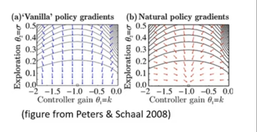
Natural Policy GradientSchulman, L., Moritz, Jordan, Abbeel (2015) Trust region policy optimization Peters, Schaal. Reinforcement Learning of motor skills with policy gradients IS objective directlyProximal Policy Optimization (PPO)
Is this even a problem in practice?
👉
It’s a pretty big problem especially with continuous action spaces. Generally a good choice to stabilize policy gradient training
With this problem, the vanilla policy gradients do point in the right direction but they are extremely ill-posed (too busy decreasing σ \sigma σ