DLS 4: CNN
Some notes of DL Specialization Course by Yunhao Cao(Github@ToiletCommander)
This work is licensed under a Creative Commons Attribution-NonCommercial-ShareAlike 4.0 International License.
Acknowledgements: Some of the resources(images, animations) are taken from:
- Andrew Ng and DeepLearning.AI’s Deep Learning Specialization Course Track
- articles on towardsdatascience.com
- images from google image search(from other online sources)
Since this article is not for commercial use, please let me know if you would like your resource taken off from here by creating an issue on my github repository.
Last updated: 2022/3/25 13:25 PST
Basic Operations
Convolution Operation
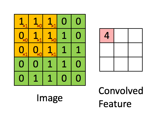
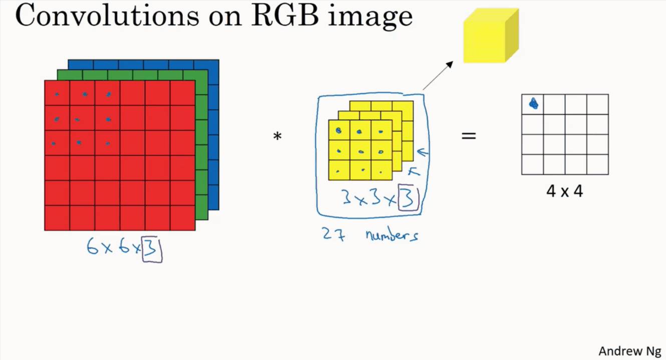
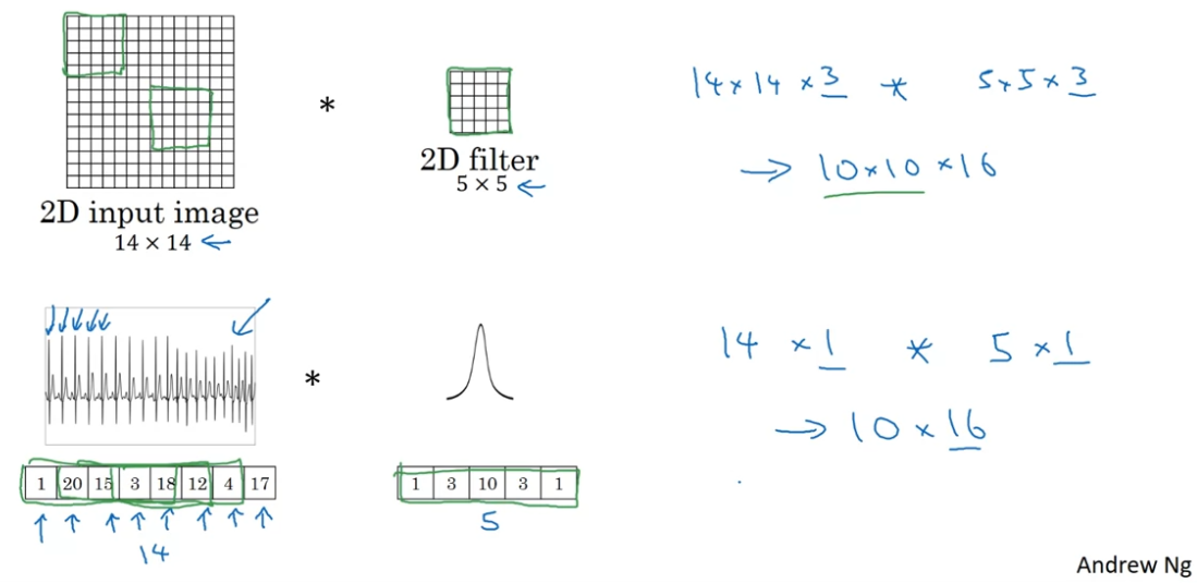
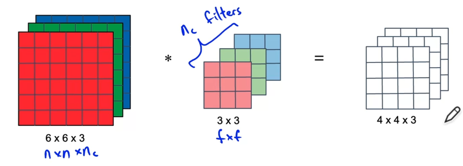
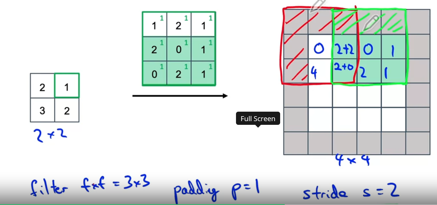
Each Convolution Filter consists of (kernel_size * kernel_size * num_channels), so the output size is determined by the number of filters in the given layer.
Also note that there’s a notion of “stride” and “padding”.
Having padding = 1 means the original input will be padded with 1 unit of “0”s on each side, so assume that the original image is w*h*c, the padded image would be (w+2)*(h+2)*c
Paddings:
- Same ⇒ Produces an output that matches w*h of the input, regardless of the kernel size of the filters
- Valid ⇒ No Padding
One by one convolution(pointwise convolution)
A way to control feature numbers
think about a convolution layer n filters of a kernel size with a stride of . This would mean that the layer preserves w*h, but changes c ⇒ n
Pooling Layers(Max Pooling / Average Pooling)
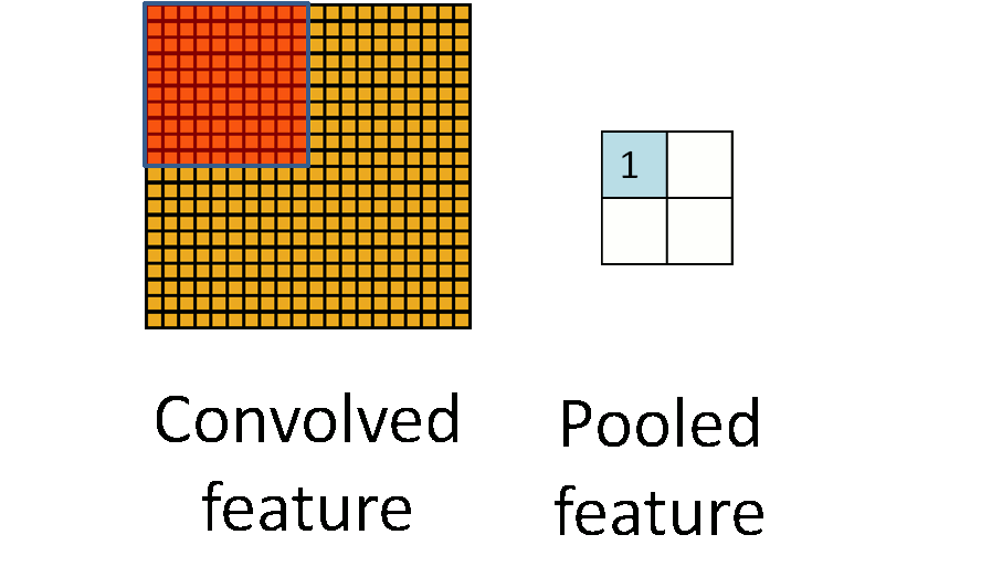
Similar to Convlution layer, the pooling layers also have a parameter on kernel size, stride, and padding(although padding is usually not used).
The Pooling Layers, instead of doing a sum on each of the operated cells, does different things
- Max Pooling simply pulls out the max value in those cells
- Average Pooling computes the average value of those cells
The intuition behind this might be:
- Pooling layers extracts features from a huge input and puts it into a lower-dimension output(shrinks w*h, not including c)
- Think about a “cat-or-not” recognizer, maybe the network doesn’t care where the cat mustache is, but as long as there is a cat mustache there’s a cat, then “max-pooling” can extract the mustache into a smaller output matrix.
Depthwise Convolution(MobileNet)
In a depthwise convolution, the number of filters is locked on to the # of channels of the input, and each filter is applied to its designated input channel. So depthwise seperable convolution does not channge the number of channels, , from input to output.
It dramatically decreases multiplications needed for each convolution operation (but of course, there’s a cost to it - performance)
Transposed Convolution(U-Net)
With U-Net, one major question is with such big number of outputs, how do you go from a small set of inputs to a large set of outputs?
- Padding is now instead put on the output layer(those ignored pads will be disgarded when outputting)
- Filters, instead of convoluting and applying on each batch of input cells, is multiplied a single input cell and applied into the “convoluting subset” on the output image
- In terms of dealing with multiple input/output channels (), the transposed convolution acts the same as normal convolution, as it assigns a tensor () for each filter.
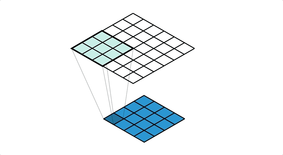
Illustration of reverse convolution, the upper layer(green) is the output layer while the lower layer(blue) is the input layer, the filter has a kernel size of 3*3 and a stride of 1

Another illustration of reverse convolution(with kernel being 3*3, stride being (2,2)), where the right(green) layer is the input layer, grey layer the applied filter with the subscript denoting the value in the filter, and left(blue) layer denoting the output layer, the dotted parts of the output layer is the padding.
Classification Networks & Bigger Building Block
ResNet → Residual Block(Skip Connections)
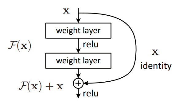
Assuming that is the activation function of layer l+2, we have...
The reason for having a skip connection is to make it easier to train bigger networks as the skip connection allows the network to learn an “identity” function
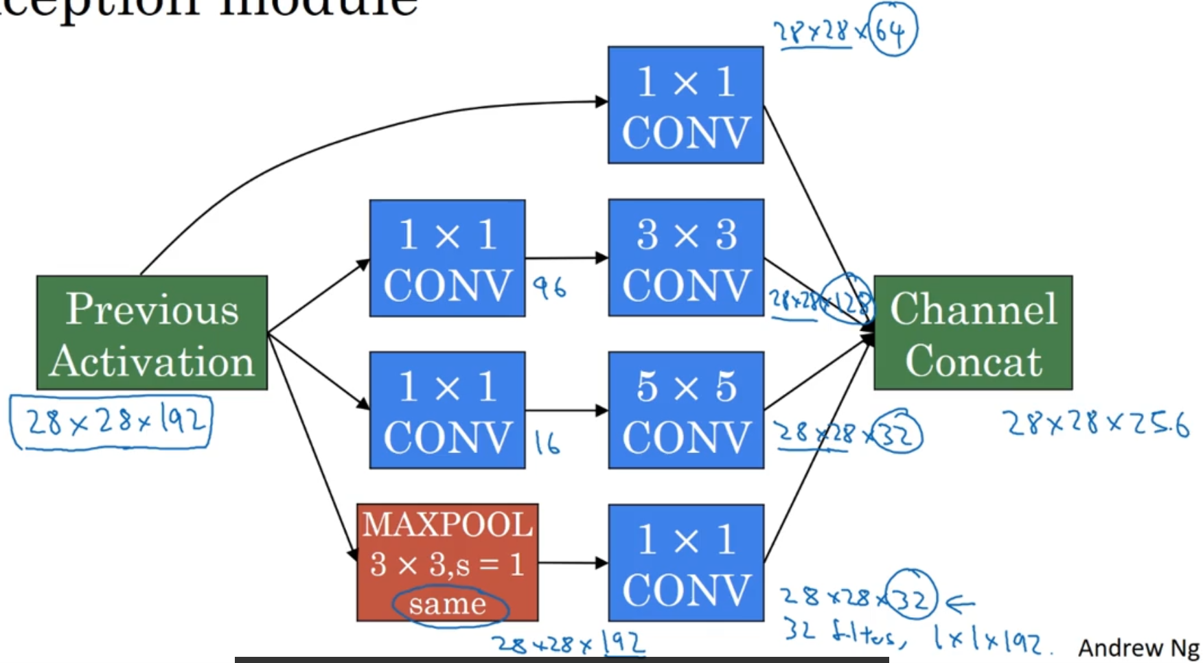
Inception Network(Inception Module)
Instead of choosing what size of conv layer / pooling layer to use, why not just do them all?
- Use ‘same’ padding for convolution & pooling to make sure the output size all match
Idea - stack each of the output on the channel axis
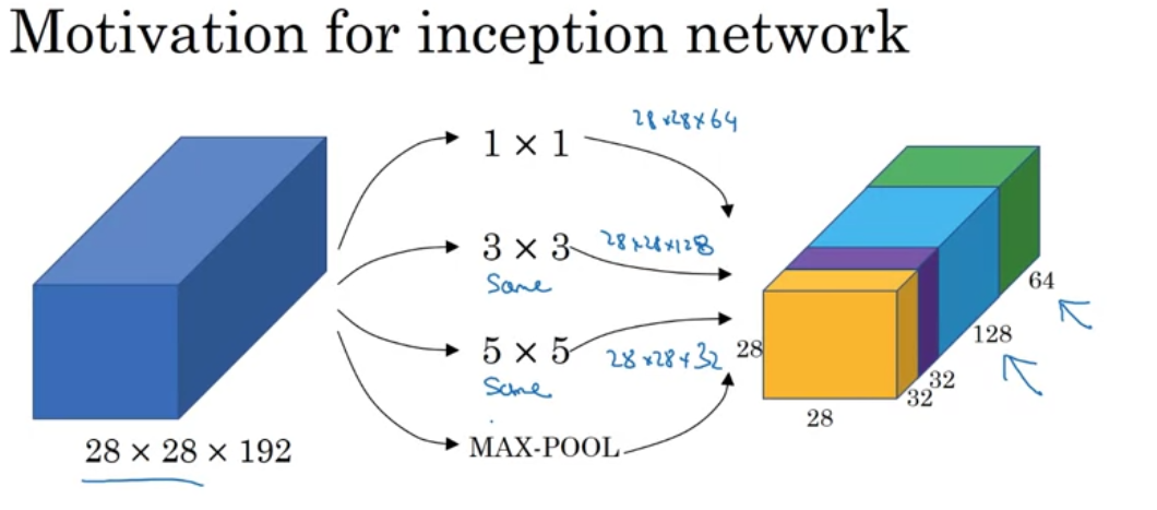
Problem is computation cost
So...
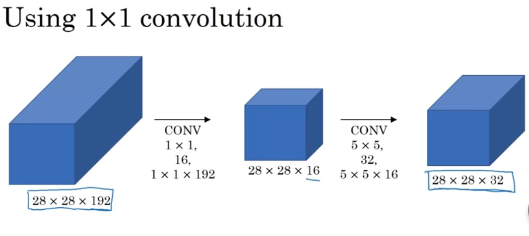
Idea is to use Conv Layer (Bottleneck Layer) to shrink the size of input layer first, then apply the actual convolution.
Final Inception Module
Note that we also apply a Conv layer after the MaxPool layer to shrink down the output size of the maxpool layer
Depthwise Separable Convolution(MobileNet v1)
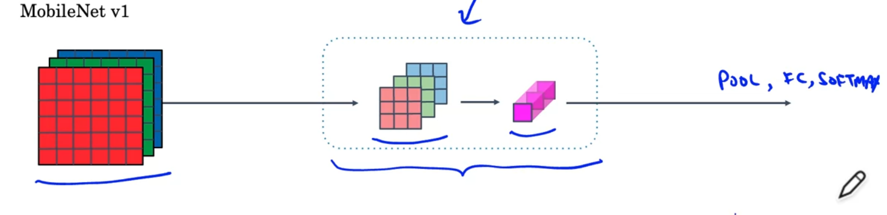
input() ⇒ Depthwise Convolution() ⇒ Pointwise() convolution()
Free to change the number of layers
Almost 10x cheaper
Bottleneck Block(MobileNet v2)
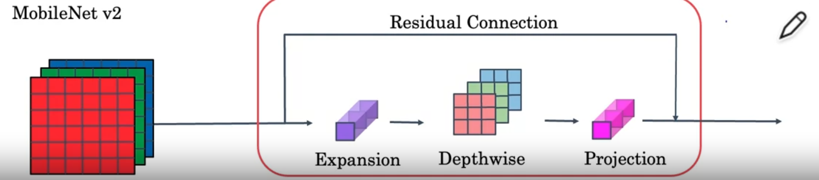
Addition of an expansion layer and a residual connection
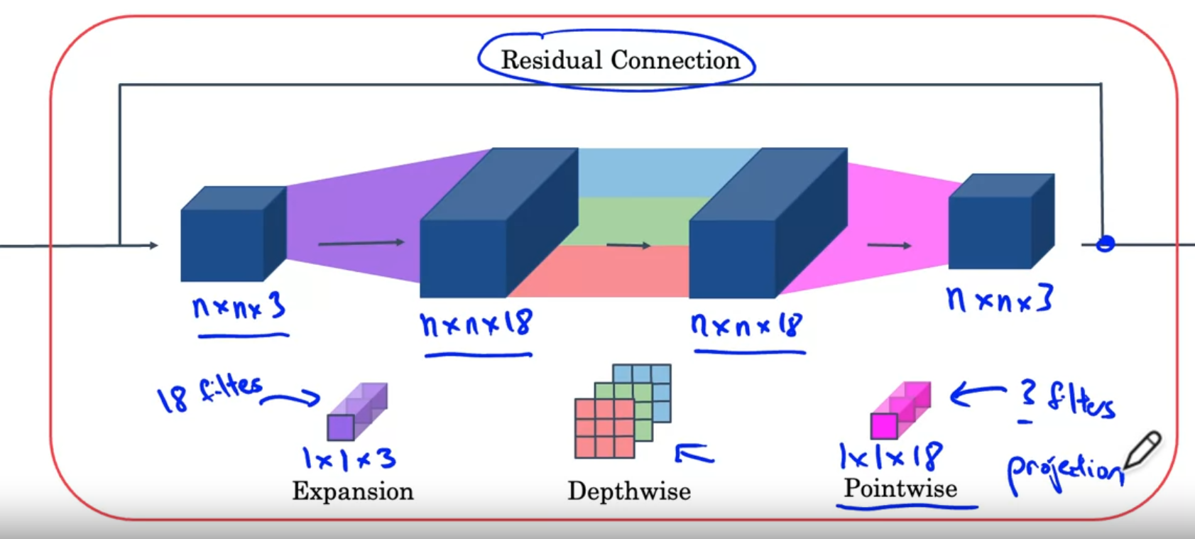
- By using expansion, increases the number of representation inside the bottlenet block
- Now it can learn a richer function
- The last pointwise(projection) operation reduces the final output and saves memory
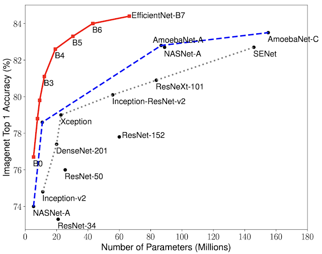
EfficientNet
Automatically scale up/down for different devices
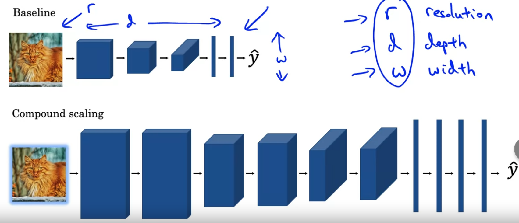
Question:
- What is the best r,d,w that has the best tradeoff between computation power and accuracy?
Unlike conventional approaches that arbitrarily scale network dimensions, such as width, depth and resolution, our method uniformly scales each dimension with a fixed set of scaling coefficients. Powered by this novel scaling method and recent progress on AutoML, we have developed a family of models, called EfficientNets, which superpass state-of-the-art accuracy with up to 10x better efficiency (smaller and faster).
Ref: https://ai.googleblog.com/2019/05/efficientnet-improving-accuracy-and.html
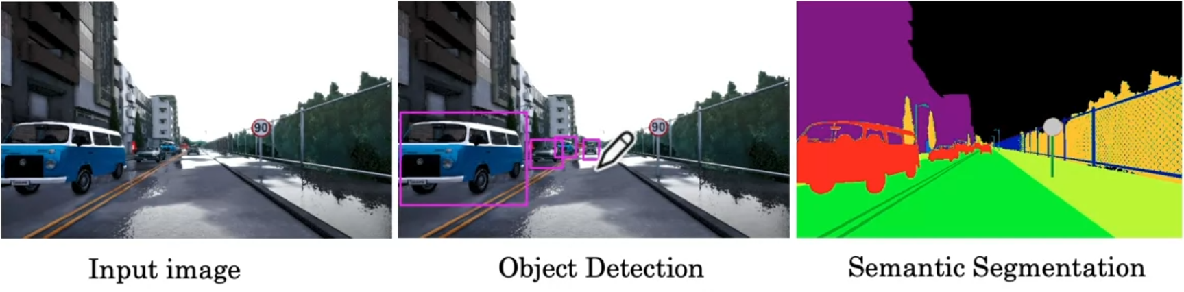
Object Detection
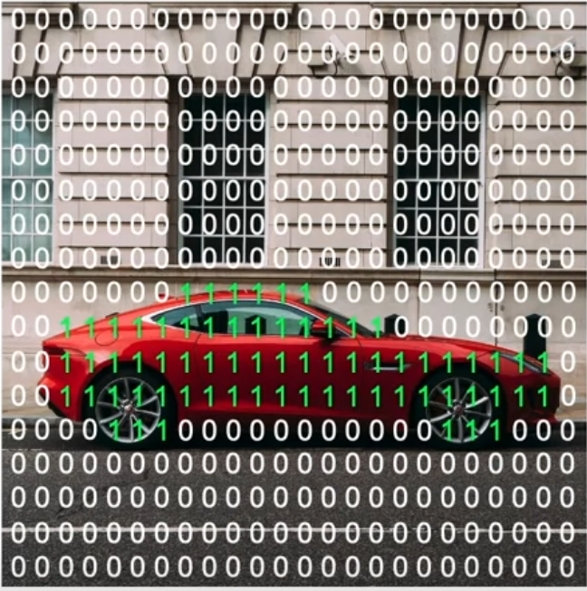
Sliding Window Algorithm
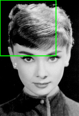
Repeatedly applying a small block filter to check if an image “contains” object, and if it does, we know there’s a object in the specific bounding box.
- Very Computationally Expensive(think about how many iterations of classification neural networks we have to go through for us to do this kind of object detection)
- Not really accurate prediction
Convolution Implemention of sliding window
Since a lof of the computations in sliding window is redundant, we can simply apply convolution layers on the “enlarged”, or “full” image
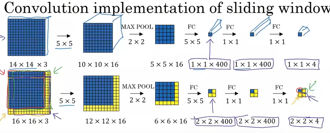
Idea of FC(Fully Connected) layer can be thought of a 1*1 kernel conv layer is pretty important here so that we can perform those FC layer on a “bigger” input from the previous layers.
YOLO Algorithm for Object Detection
Algorithm Basics
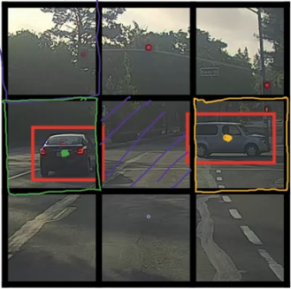
First split the image into multiple sections
In this example the image is splitted into parts, but in practice we usually use a finer grid such as to train a YOLO(You-Only-Look-Once) network.
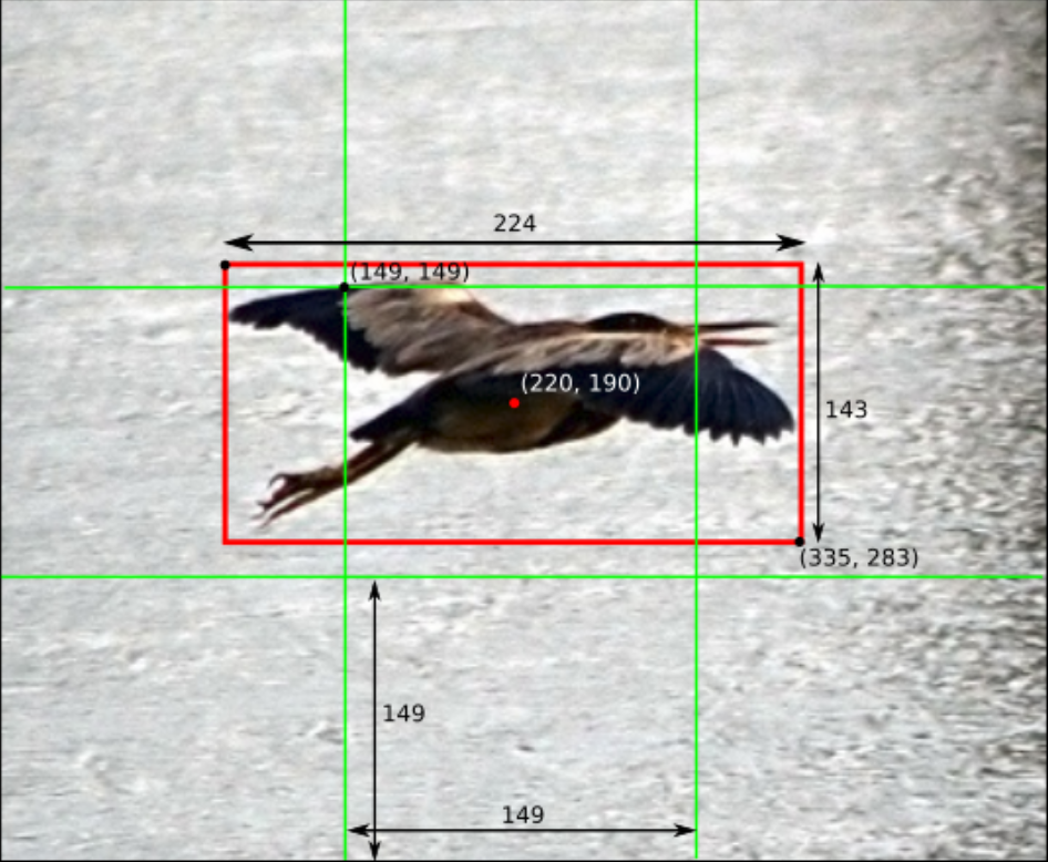
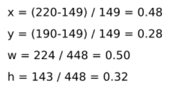
The prediction result for each cell(small part) is:
where each denotes the prediction results for the anchor boxes, where:
and
Note the difference between the notation of and , they mean different things
In here,
 https://stackoverflow.com/questions/52455429/what-does-the-coordinate-output-of-yolo-algorithm-represent
- denotes the probability that there is an object in this anchor box
- If in the training example, then the remaining values, including , should be (don’t care), which means there should be no punishment on the cost function on those values, only a wrong would get the network punished.
- denotes the position of the center of the bounding box, where denotes the top-left corner of the grid cell
- It is not possible for to exceed the limits as each grid cell is only responsible for the object that has its center being contained.
- has two interpretations
- , and it can be interpreted as, the fraction of width and height of the entire image ⇒ USED MORE OFTEN
- normalized but can exceed 1.0 ⇒ interpret it as the fraction of width and height of each grid cell.
Expanding on the definition of Anchor Boxes
Anchor Boxes allows each cell to detect multiple objects...
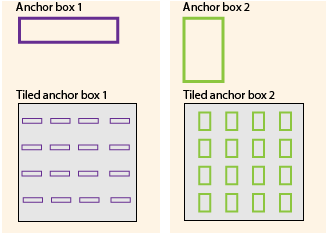
Anchor boxes are a set of predefined bounding boxes of a certain height and width. These boxes are defined to capture the scale and aspect ratio of specific object classes you want to detect and are typically chosen based on object sizes in your training datasets.
The network does not directly predict bounding boxes, but rather predicts the probabilities and refinements that correspond to the tiled anchor boxes.
Concept of IOU(Intersection over Union)
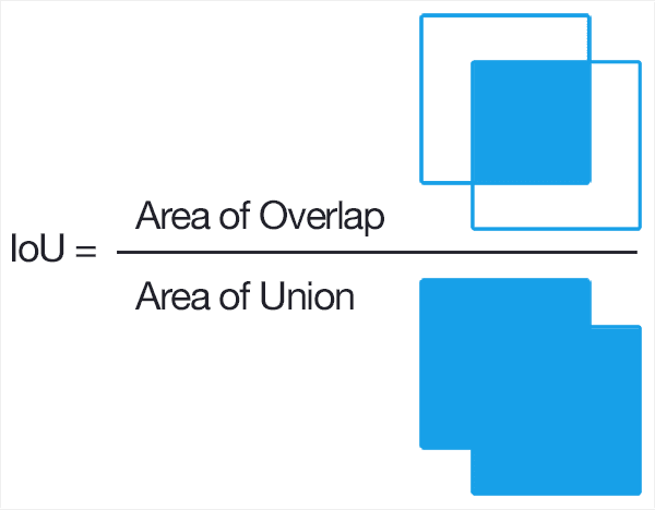
Computes the fraction of overlap between A and B
This concept becomes very handy when doing non-max supression.
Non-max Supression
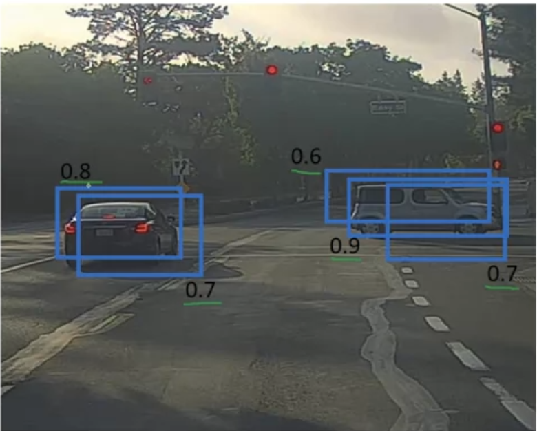
Sometimes a YOLO model can predict an object with overlapping bounding boxes, and non-max supression helps you to gain a much clearer prediction result.
Steps:
- Suppress ALL boxes with
- We want GOOD predictions
- Pick max and supress non-max
- First highlight the bounding box with the max probability
- Find the IOU of this bounding box with other bounding boxes (with the same class)
- If the , then eliminate the other bounding box
- If not, then leave the other bounding box
- Repeat the first step on the second max probability, third...until we found all rectangle to have either been passed through or eliminated out.
R-CNN(CNN with region proposals)
stands for Regions with Convolutional Neural Nets
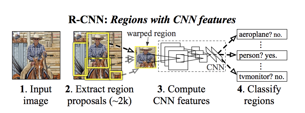
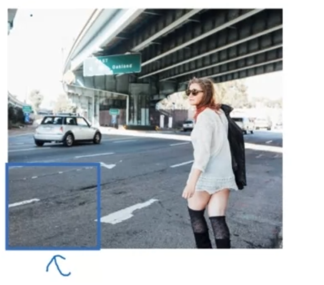
The downside of Convolutional Sliding Window is you spend some time trying to detect an object from a sub-part of the image that clearly doesn’t have an object, say this one...
So instead of using a sliding window, let an algorithm(With R-CNN, its called a segmentation algorithm) propose a few regions and we just run our classifier on those few regions.
After proposing, R-CNN output a label and a bounding box. Note that the bobunding box can but doesn’t necessary have to be the bounding box the segmentation algorithm proposes, it actually trys to figure out a better bounding box.
Turns out that this is still slow...So work has been done to try to speed up this algorithm
| R-CNN | Propose Regions. Classify proposed regions one at a time and outputs label + bounding box |
| Fast R-CNN | Propose Regions. Use convolution implemention of sliding windows to classify all the proposed regions. |
| Faster R-CNN | Use CNN to propose regions. |
Andrew NG: He thinks YOLO is a better algorithm than any R-CNN implemention. Even the “Faster R-CNN” is a bit slower than the YOLO. (doesn’t represent the entire CV industry)
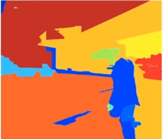
Semantic Segmentation
Draw a careful outline for objects detected so you know exact which class each pixel belongs to.
U-Net
Small Intuitions(Simple Diagram)
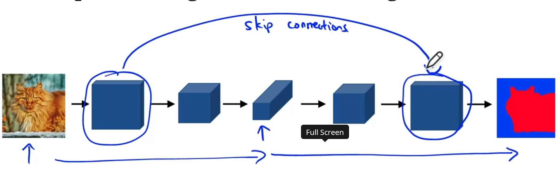
The skip connections is not directly applied with what the residual block does, instead it simply concatenates the result of last block with the result of a very previous block
Why does the skip connection make sense?
- semantic segmentation requires two types of data, one from low resolution, high level contextual information (from the last layer) and high-resolution, low-level-feature information (from earlier layer) to determine if each pixel belongs to a class or not.
Actual Architecture
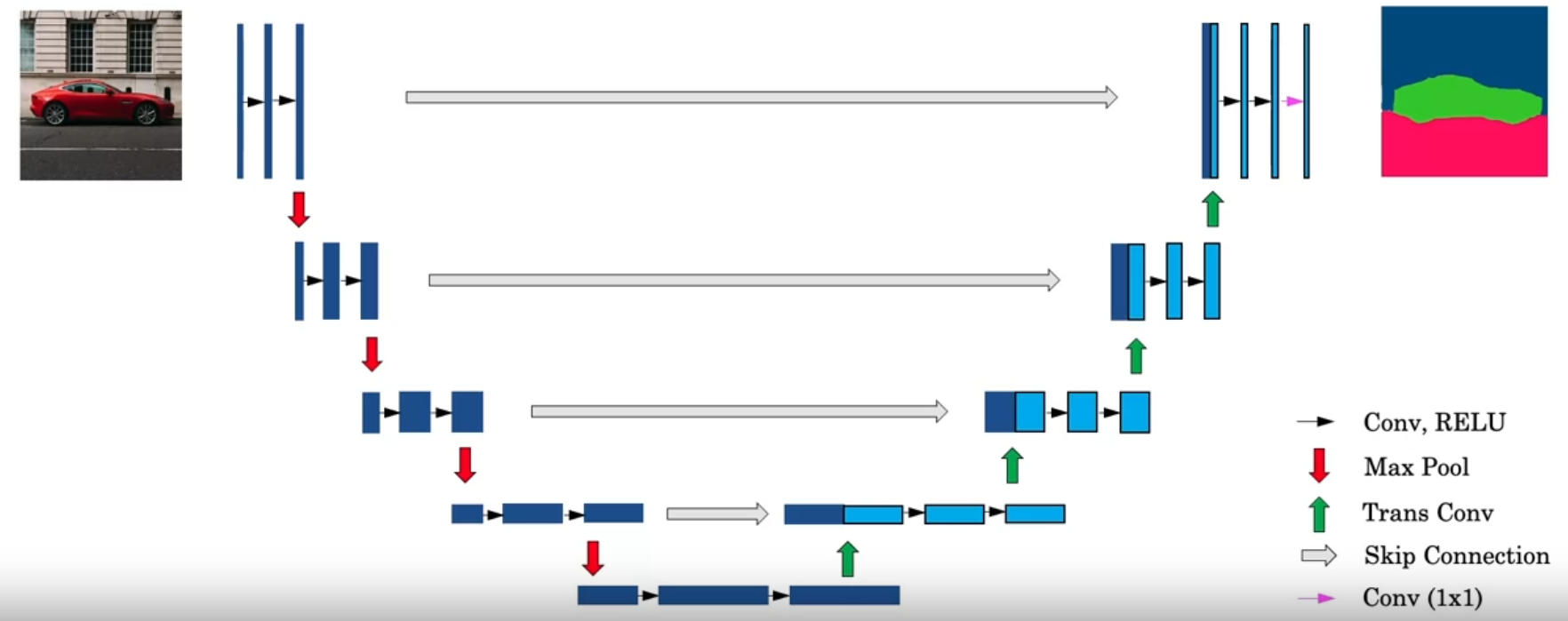
For the first blue “bar”, imagine the image as this thin bar of layer
Think each of those bars as their height as , while their width as (number of channels)
The “downward” layers uses normal set of Convolution + Relu layers
As the “height”() of the layers gets small(usually the is increased by a factor of two for each downward), start to use tranposed convolutions, denoted by the green arrows, with each transpose convolution operation followed by a concatenation of “skip connection”(takes the left, dark-blue output portion and concatenate to the front of the output of the trans conv, on the right of the skip arrow)
After transconv, apply a couple more layers of conv ⇒ relu, then apply trans conv again...
Keep increasing the height(usually the number of downward = number of upward, and the size of transpose conv and the downward pooling are the same to make sure that the returned w*h are the same as input, and each time we go up, typically is halfed)
After the “height” reaches the original “height”, use of conv to make sure the
One-shot Image Recognition
In a face-recognition program we want to learn about a person’s face once and be able to recognize them in the future. This is called one-shot image recognition problem, because we have relatively little data to “train”(called anchor image). One plausible approach will be to use a “difference” function that compares the “distance” of two images(one “training/reference” image(anchor) and one “test” image(positive/negative)).
Siamese Network(DeepFace)
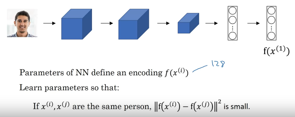
Instead of outputting a softmax layer in the end, output a feature vector
Train to minimize if are from the same person, and maximize if are from the different person.
In the above picture, is difined as .
Triplet Loss (Loss Function) [FaceNet]
A loss function for siamese network to use...
Objective:
Minimize
Constraint:
But we don’t necessarily want this to be 0, why? Because the algorithm can just learn to output the feature vector as all zeros(or all images with the same output, causing N-N = 0), so we can add a margin variable
So...
The max function serves as, if our objective is negative, the loss function is 0 (Since L has to ≥ 0), but if the objective is positive, it outputs the objective function value.
Training Set
Training Set still has to be big....10k images for 1k people maybe.
After training, apply it to one-shot problem.
It is important to choose the triplets, A, P, N though.
If A, P, N are chosen randomly, it is pretty easy to satisfy the constraints.
So choose triplets that are “hard” to train on - maybe find similar-looking people?
One-shot Recognition as a classification problem
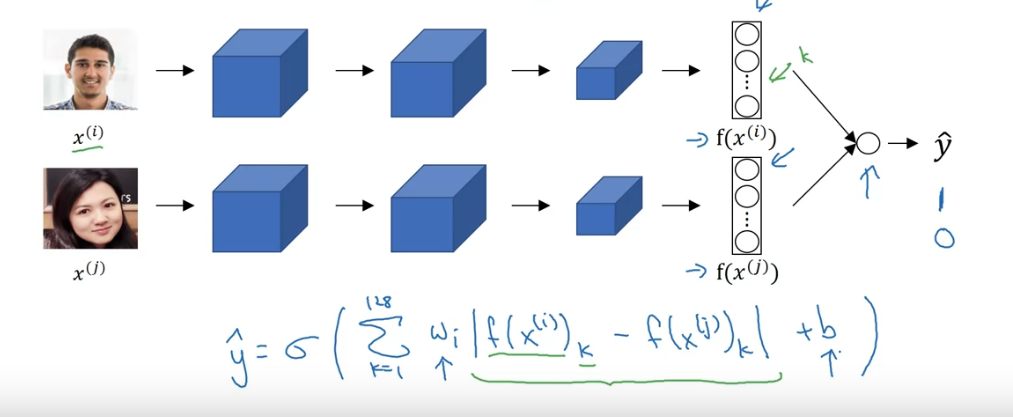
So this time connect the output of our “Siamese Network” and connect the two vectors into a logistic regression unit, the input to the logistic regression unit can either be modified or not, based on your choice. (The image on the top takes a sum of element-wise absolute vector as the set of input to the logistic regression unit).
Note parameter of the two “Siamese Network” are the same...
here is output by a sigmoid function to produce a “probability” estimation.
Possible Input Methods:
“absolute similarity”
“chi square similarity”
Other variations are explored in the “DeepFace” paper
Visualizing what Deep ConvNets are learning
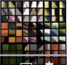
On the left picture, we have a convnet and on the right each nine pictures that make a square block represents nine image patches that maximizes the unit’s activation.
Pick a unit in any level, find the nine image patches that maximizes the unit’s activation. Tells you what each unit is trying to find.
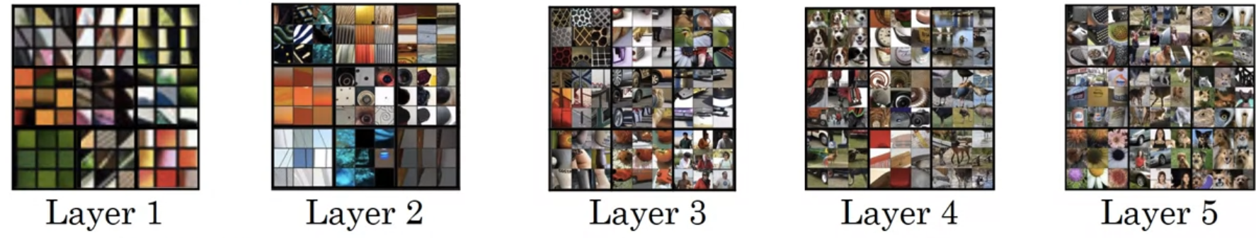
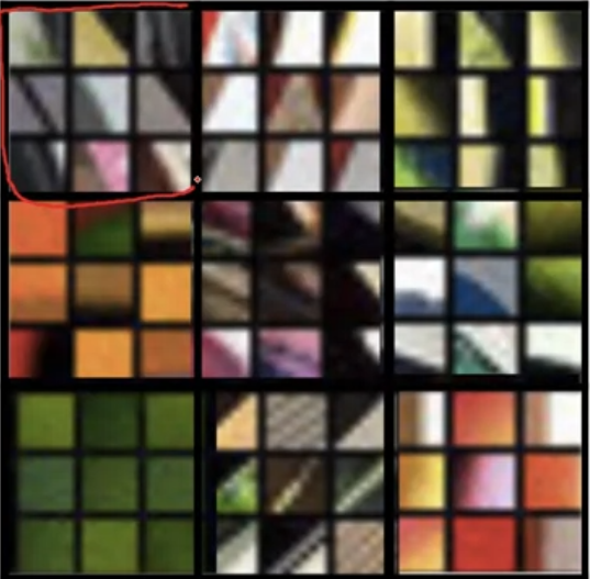
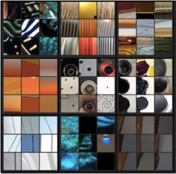
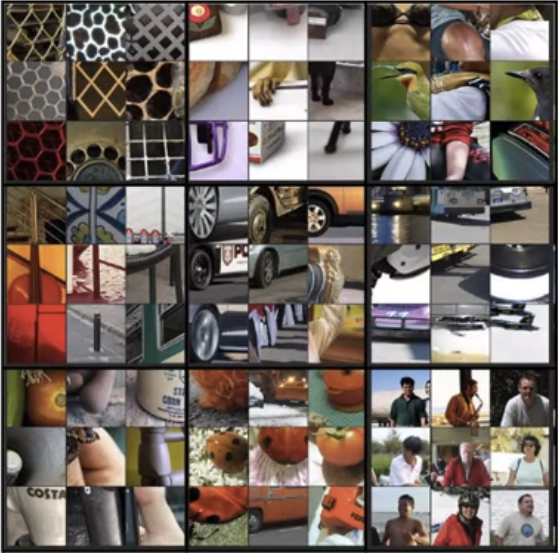
As we go deeper and deeper in layer, it seems like the deeper layers are detecting more complex (high-abstract) features.
Neural Style Transfer
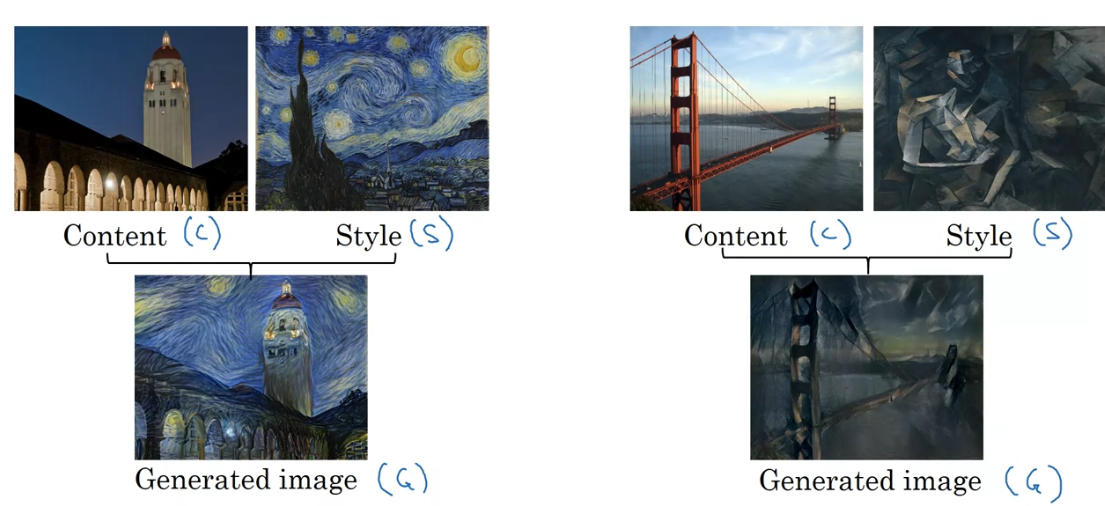
Given a content image, and an image of “style” reference, generate an image of the content image with the style similar to the style image
Cost Function
Content Cost Function
- Say you use hidden layer to compute content cost (l not too deep not too shallow)
- Use pre-trained ConvNet (e.g. VGG Network)
- Let be the activation of layer l on the image
- If are similar, then both images have similar content
Style Cost Function
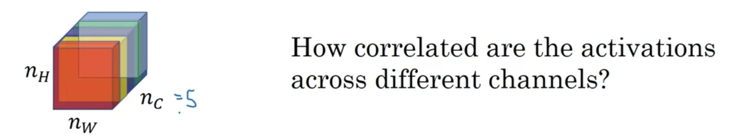
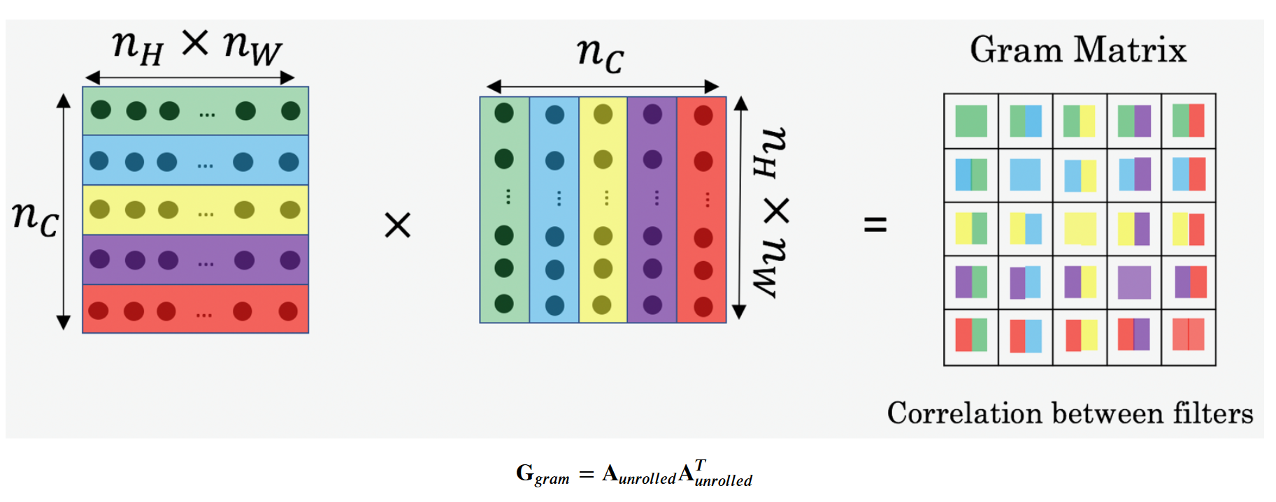
Define “style” as correlation between activations across channels
So compute the “style matrix”, which measures all correlations between different channels
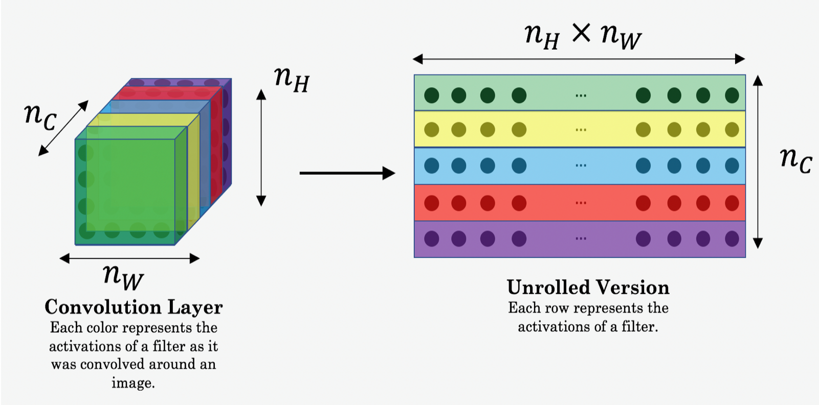
Let be the activation at (i,j,k). Note i,j,k corresponds to height, width, and channel respectively.
We will compute a gram matrix , which is in dimension ⇒ measures how correlated the activations in channel k is correlated with the activations in channel k’
The normalization constant is just used in the author’s paper...but not necessary since we have a constant in the overall cost function
It turns out its best if we use the style cost function from multiple layers...so we’ll just sum over all layers.
The parameter allows you to adjust weight for each layer’s style cost function.
Find the generated image G
- Initialize G randomly ()
- Use gradient descent to minimize ⇒
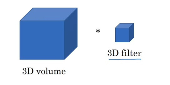
Generizing the concept of ConvNet to 1D/3D Image