Some notes of DL Specialization Course by Yunhao Cao(Github@ToiletCommander)

This work is licensed under a Creative Commons Attribution-NonCommercial-ShareAlike 4.0 International License.

Acknowledgements: Some of the resources(images, animations) are taken from:

1. Andrew Ng and DeepLearning.AI’s Deep Learning Specialization Course Track

2. articles on towardsdatascience.com

3. images from google image search(from other online sources)

Since this article is not for commercial use, please let me know if you would like your resource taken off from here by creating an issue on my github repository.

Last updated: 2022/3/25 13:25 PST

Why Sequence Models

So it seems like we’ve learned enough of our fixed-size and fixed-size output neural nets, its time to think about when the inputs and outputs would not match.

Due to limitations of neural architectures, it seems like the computer only accepts fixed-sized inputs and fixed-sized outputs. The structure of this kind of neural nets makes it easy to accept fixed-structure inputs and fixed-structure outputs.

But consider if we want to transcript an audio clip into a sequence of text, in which case both input and output can be different in length each time.

So what now?

Solution is to use sequence models

Notation

Note that we are feeding fixed-length structured data into the same model recurrently.

$x^{<t>}$ denotes the t-th sequence input, t starting from 1

$y^{<t>}$ and $\hat{y}^{<t>}$ denotes the t-th sequence label and output, respectively, t starting from 1

and $T_x$ denotes the length of the input sequence, where $T_y$ denotes the length of the output sequence

$x^{(i)<t>}$ denotes the t-th element in the input sequence of the i-th training sample

$y^{(i)<t>}$ denotes the t-th element in the output sequence of the i-th training sample

$T_x^{(i)}$ denotes the length of the input sequence of the i-th training sample, and $T_y^{(i)}$ denotes the length of the output sequence of the i-th training sample

Recurrent Neural Network (RNN)

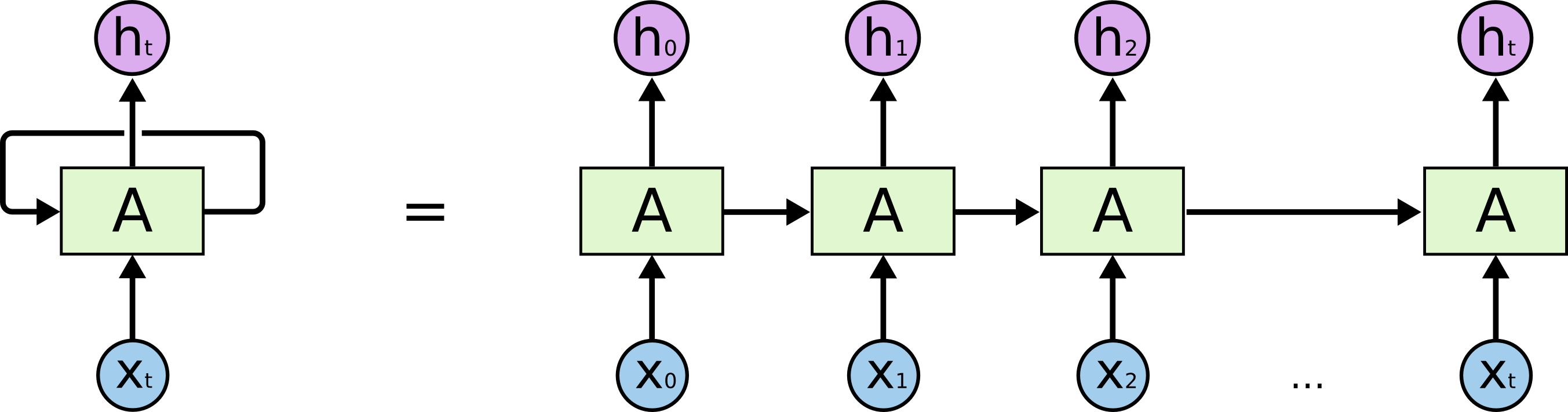
The recurrent neural network is different from a normal NN structure such that it also accepts a $w_{dd} \cdot a^{<t-1>}$ input aside from $x^{<t>}$ ⇒ So that the information from previous inputs is passed into the network.

However, there are some short-comings of this structure

1. Magnitude of information from the inputs from really early on will gradually decrease as we progress through series of inputs in the sequence.

2. The NN doesn’t have any information about what is happening later on.
   1. Introduction of Bidirection Recurrent Neural Network(BRNN) later on.

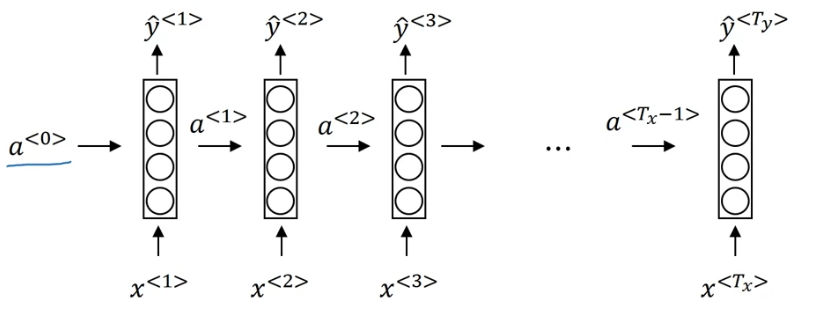
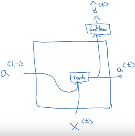
Forward Propagation

$a^{<0>} = \vec{0}$

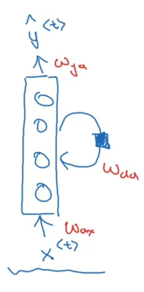
To simplify this activation calculation,

where...

Different Architectures(Or forms) of RNN

Sequence Generation & NLP with RNN

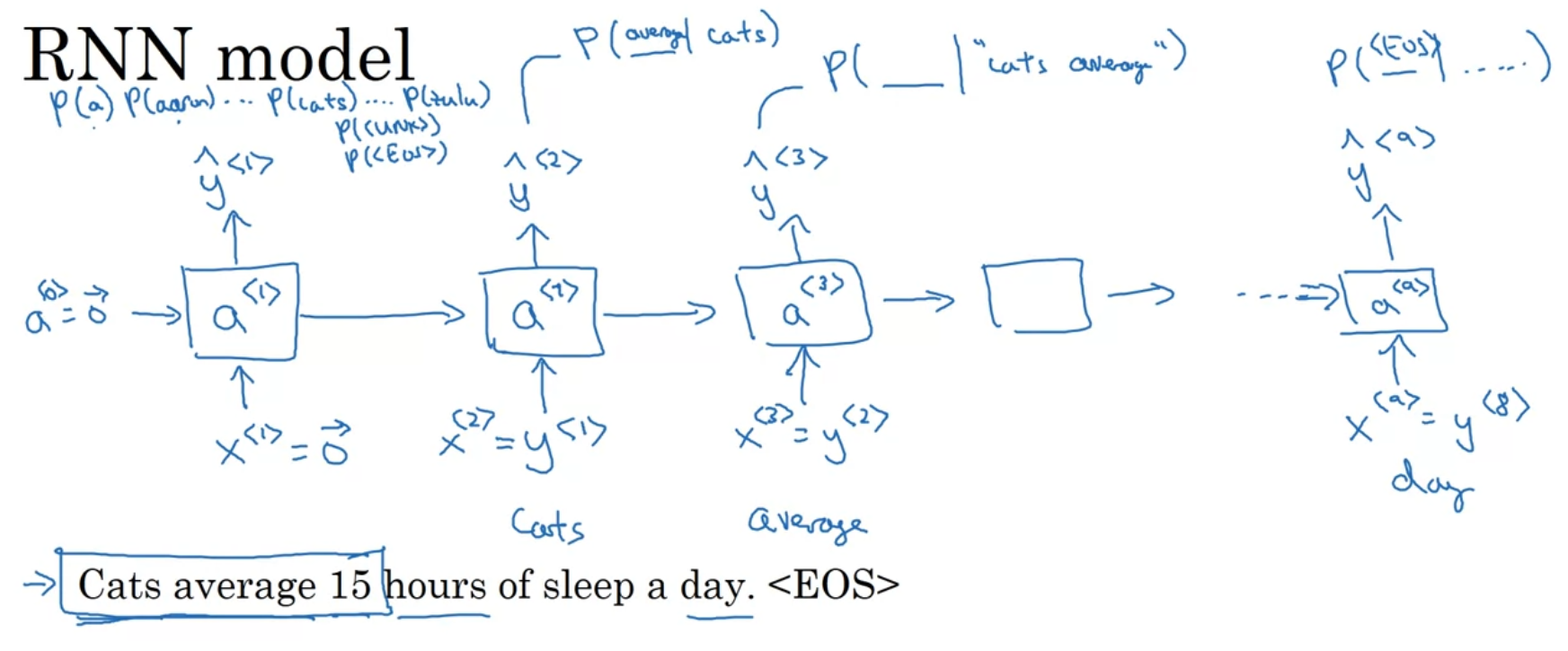
We assign each vocabulary with an index, so we would have a max index of $\text{vocab\_num} - 1$. Each time we pass in a word, we would pass in a one-hot vector $\vec{v}$ representing the word, with the $i$th element being 1 and the other elements of the vector being zero. $i$ would be the index of the word.

Note that we will introduce other ways to represent words later.

Output of $y^{<t>}$ would be a softmax output layer with also $\text{vocab\_num}$ long vector output. Each index of the vector represents the likelihood of a specific word that follows.

Training

Sequence Generation Loss Function:

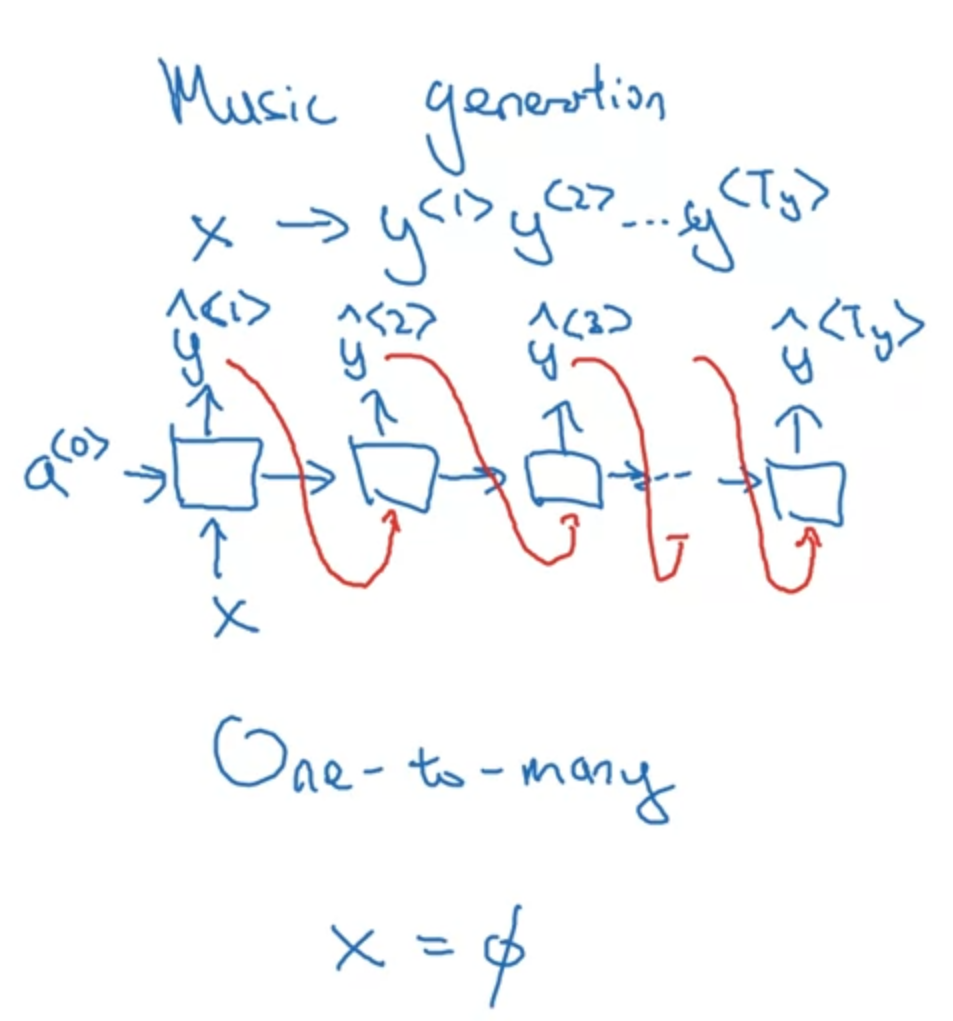
Generating Sequences

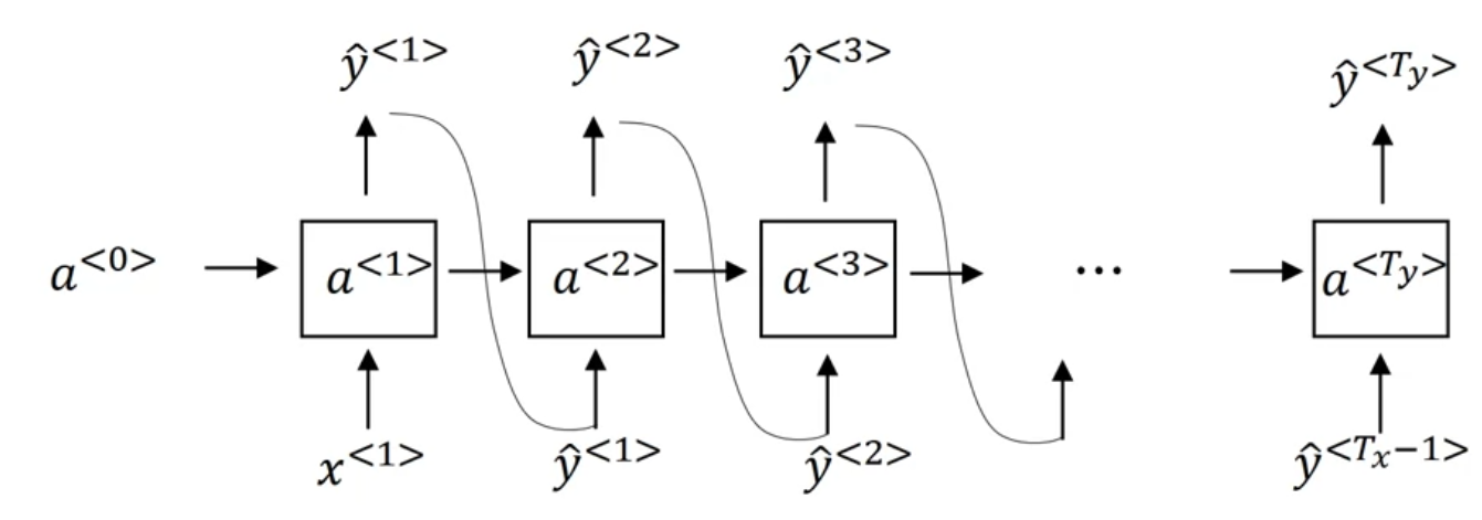
As we did before, pass in $a^{<0>}$ and $x^{<1>}$ as zero vectors

For each $\hat y^{<t>}$ that outputs the possibility of each word(a vector representing the possibility of each word) given the input of $x^{<t-1>}, x^{<t-1>}, \dots, x^{<2>}$, we would sample a word index by using the probability distribution given by $\hat y^{<t>}$, and assign it as $x^{<t+1>}$. We stop until we hit the index of <EOS> or arrive at a limit.

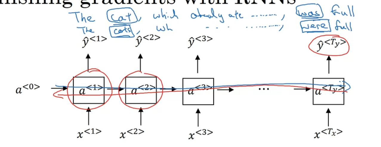
Vanishing Gradient with RNN

Think about the following two sentences

1. The cat, which already ate ....., was full.

2. The cat, which already ate ....., were full.

Problem is original RNN is not good at capturing long-term dependencies. See below as it is hard for the gradient to propagate through so many connections.

Bidirectional Sequence Model (Bidirectional RNN/BRNN)

Note: Works on any sequence unit like GRU, LSTM, RNN, etc.

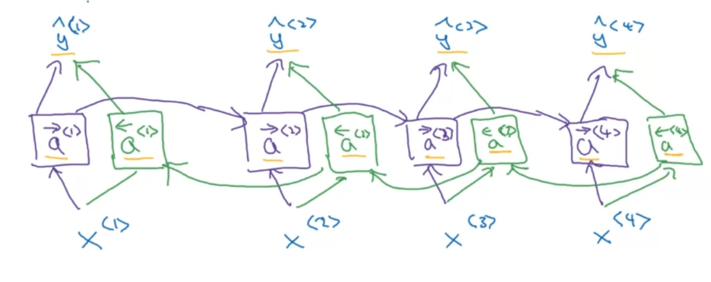
Need entire sequence of data to process data, so if used in a speech recognition, we need the person to stop talking to start dealing with data.

Deep RNN

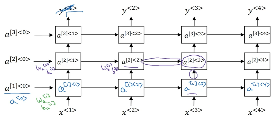
See now that we can stack units of RNN, GRU, or LSTM layer by layer (from bottom to top) to form bigger neural networks. We can also add dense(FC) layers after those sequence model layers.

Gated Recurrent Unit (GRU)

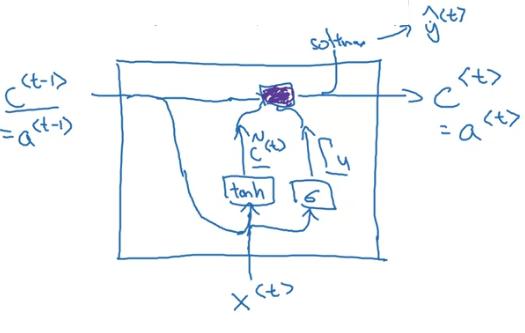
Addition of new $c^{<t>}$(cell of memory) here(althogh $c^{<t>} = a^{<t>}$, but later in LSTM they would be different).

Long Short Term Memory(LSTM)

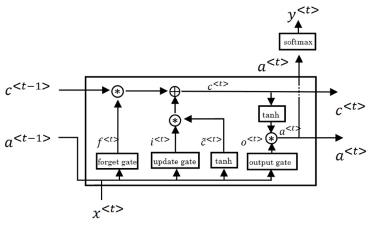
Now note that now $c^{<t>}$ and $a^{<t>}$ both represents different things.

Note: Andrew Ng Used $g_a(x)=g_c(x)=tanh(x)$

Word Embeddings

Remember early in the Sequence Generation RNN models we used one-hot vectors to represent our input words? We can instead use word embeddings to represent our words.

Now our input would still be a vector. This vector would now represent...

Note that now we no longer add the index of the word to the input. We’ll use word embedding vectors instead.

Representation

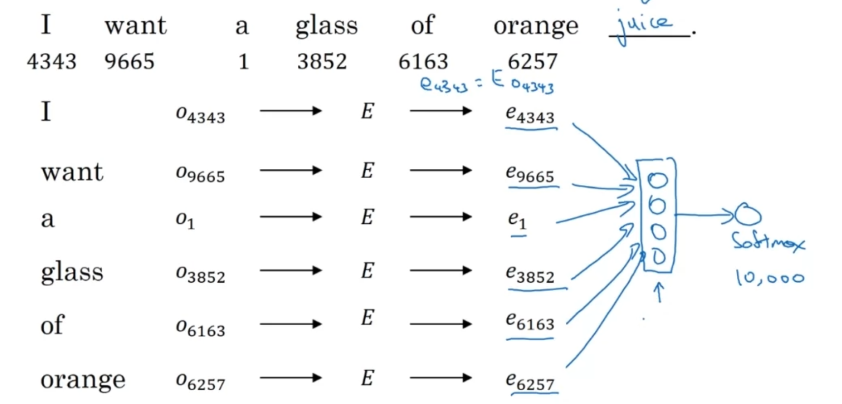
We will use an embedding matrix $E$ which each column $\vec e_i$ represents the embedding of one word. This is so that when we take product of $E$ and $\vec o_i$, $\vec o_i$ representing the one-hot vector of word i, then $E\vec o_i$ represents $\vec e_i$, the word embedding for that specific word.

However in practice we would never use the embedding matrix to find the embedding of the word(to avoid computation overhead). Instead embeddings are stored in rows for easy index retreval.

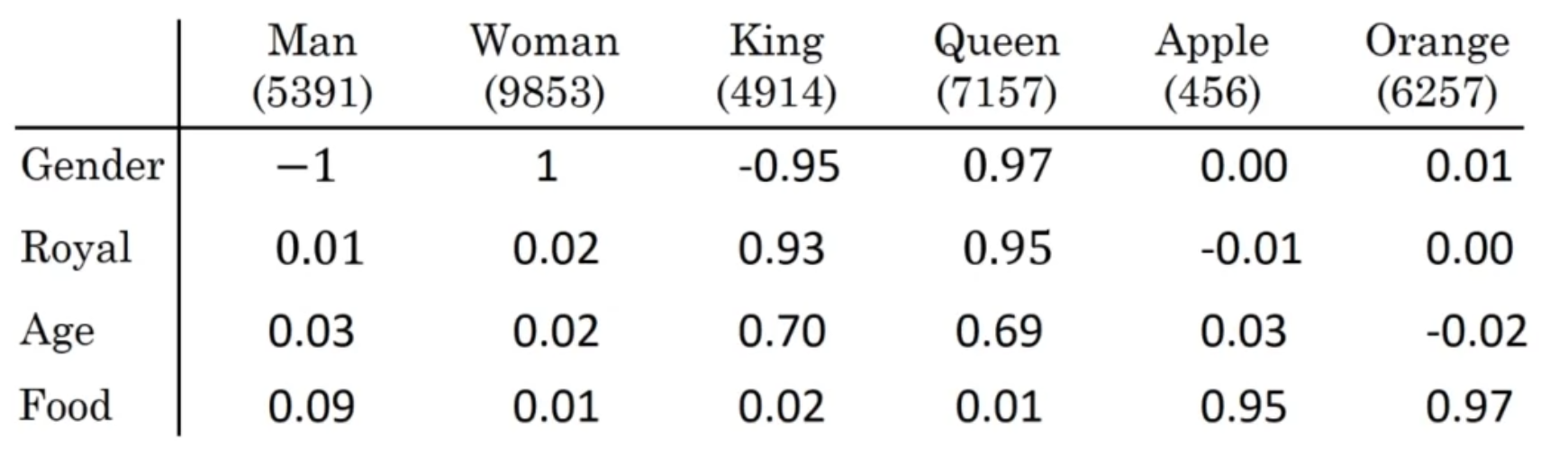
Calculating Analogies

Let $\vec{v}_{man}$ be the vector representing word “man”, we want to ask the following question:

Man to King is as Woman to ?

The answer to the question mark is of course queen.

To find the answer, we can use embeddings to find the closest word, represented by $\vec{v}_{?}$, such that

is minimized.

There are lots of ways to calculate the distance, we will introduce two.

Methods for Learning Word Embeddings

So now instead of using word embeddings as an input, while training word embeddings, we would actually add an embedding layer to the model so that the algorithm can optimize it. Our input will now be reverted back to one hot vectors(stacked together) and we would multiply it by the embedding matrix $E$ in the embedding layer. Notice that $E$ can be optimized.

Dumb Method

Learning Goal: To provide great embeddings for words.

Learning Task: Predict the probability of a word given some context words (like 5 words before, or 5 words after, or ten words before and after, last one word, nearby one word etc.)

Model: FC layers connected with a softmax layer. No RNNs are used.

Loss: $L(y,\hat{y})=-\sum_{i=1}^{vocab\_size} y_i log(\hat{y_i})$

To sample the context c,

If we do this uniformly at random, we will find that we will see words like “the, of, and, to” appearing much more frequently than other words

Word2Vec

Use a context word and a target word to train a softmax output neural network.

Negative Sampling

For softmax classification, we used the following formula.

But this will be very computationally heavy when $vocab\_size$ gets big.

We can use a hierarchical softmax layer or use negative sampling.

With negative sampling, instead of outputting a softmax vector, we will use a sigmoid activation function to predict the likelihood of two words being an context-target pair.

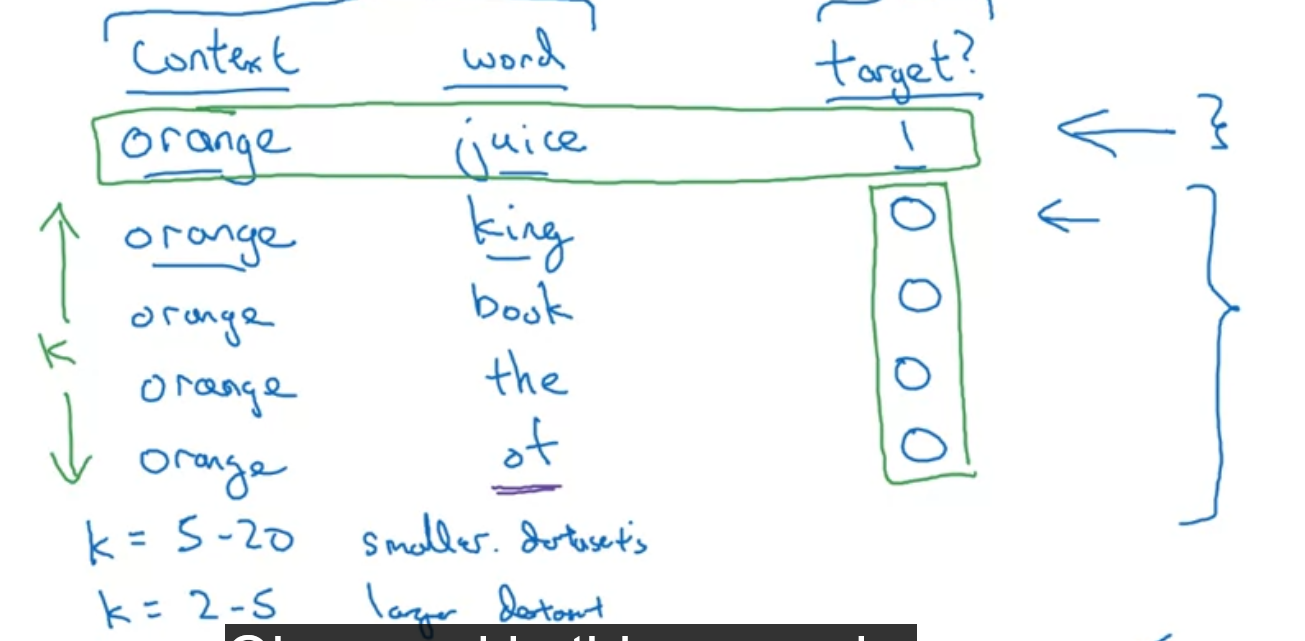
Generate positive samples by sampling sentences and generate negative samples by randomly choosing and placing words together.

Glove Method

Global Vectors for Word Representation

Lets say that $X_{ij}$ denotes the number of times in the sample such that word j appears in the context of i.

Depending on how the context is solved, $X_{ij}$ might be equal to $X_{ji}$

The glove method tends to minimize the following weight...

Here $f(i,j)$ is a weighting function such that

Notice here that $\theta_i$ and $e_i$ has the same role mathematically, what we usually do is when we need our actual “trained embeddings”, we would take $e_i^*=\frac{e_i+\theta_i}{2}$.

Neutralizing(Debiasing) Word Embeddings

Our texts to train word embeddings might include words that include stereotypical assumptions. So we want to neutralize them.

How?

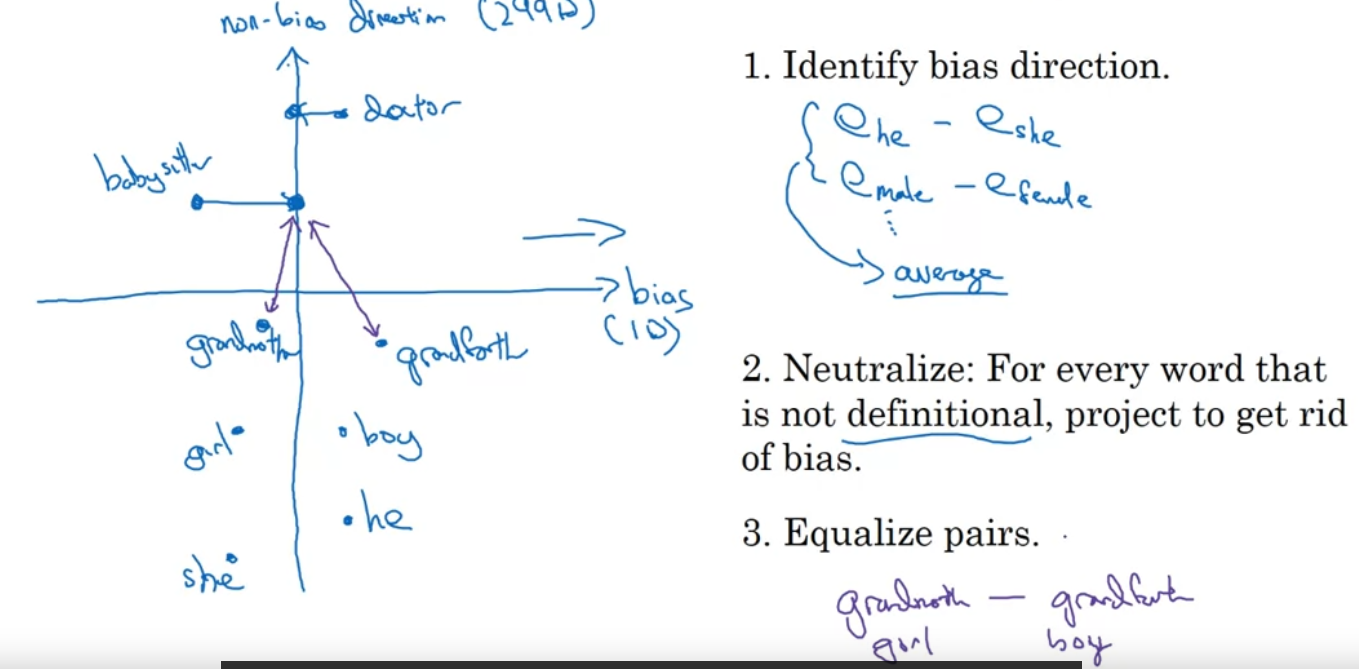
Say for example that we want to neutralize words that involve gender bias.

1. Identifying Bias Term: First we need to calculate the “bias vector” $v_{bias}$, that would be the basis vector representing the bias.
   1. We would take a few word pairs representing gender and average their difference, for example, we average over $e_{boy}-e_{girl}, e_{man}-e_{woman},e_{king}-e_{queen}$, etc.

2. Neutralize: Then for every word that is not definitional, for example, $e_{k}$, we project $e_k$ onto $v_{bias}$ and get rid of the projection from $v_k$
   1. Example of this would be occupations, there’s no gender involved.

3. Equalization: For words that are pairs in gender, we want to make sure that all of their differences are gender

Translation and Voice Recognition

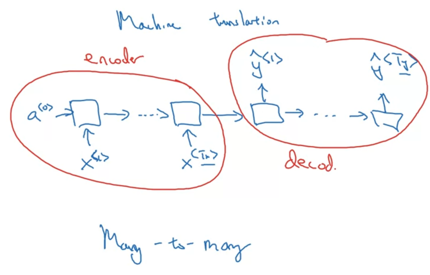
Basic Encoder Decoder Model

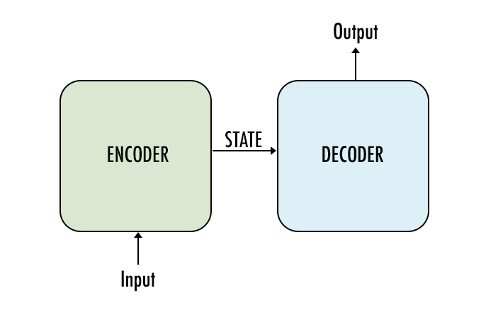
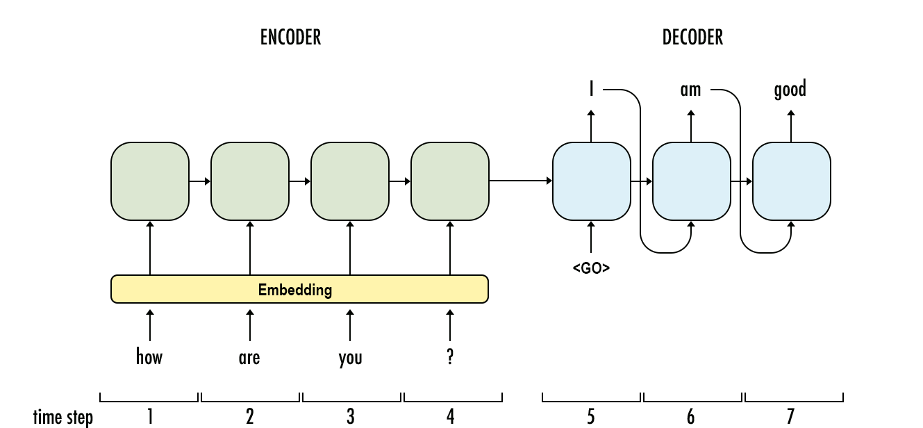
This is the basic encoder-decoder model where sequences are first inputed into the model and processed and then passed as an intermediate activation state to the second part of the model. This model works for small or short translation tasks but due to information loss will not be able to perform well on long inputs.

Picking the most likely word or sentence(Beam Search)

In the above model, during the decoder phase, every element in the $\hat{y}^{<t>}$ output vector gives probability of the following: $\mathbb{P}(y^{<t>}=i | x^{<1>},x^{<2>},\dots,x^{<n>},y^{<1>},y{<2>},\dots,y^{<t-1>})$

So we want the most likely word or sentence, we want to maximize the likelihood of the whole sentence. Let our choice of y hat each time being the $i_t$ element of the output, then we want to maximize $\prod_{k=1}^{t}\hat{y}_{i_k}^{<k>}$

We can search through the output by using a greedy algorithm, but that’s just too computationally expensive. So instead we will use a heuristic search algorithm called beam search.

Beam Search has a parameter, beam width $\beta$, that limits how many choices it can keep. It is basically a BFS with limited numbers of selection to hold while each time we propagate through the sequence.

Error Analysis in Beam Search & NN

Note that when we employ beam search, it might be hard to detect whether error comes from the neural net or the search algorithm. If we’ve selected $\hat{y}$ while the optimal solution should be $y^*$, it is usually useful if we inspect the output of the neural net and calculate $P(\hat{y})$, and $P(y^*)$ accordingly.

If we compare them and find that the neural net outputs $P(y^*) > P(\hat{y})$, then we know the beam search didn’t find a better solution even though the neural net was correct. So we might need to increase beam width $\beta$.

Otherwise $P(y^*) \le P(\hat{y})$, then we need to improve the NN since the NN is not giving the optimal solution a bigger weight.

Bleu Score

Bleu Stands for Bilingual Evaluation Understudy.

Basic Idea: Given input x and some reference output ys, we can compare our NN output with the reference ys and determine how many words overlap with the reference, and this will somehow give us the quality of our output.

Note that here we have multiple y because different people might have different translation of the same text.

Here we will first define some vocabularies:

n-gram: one(n=1) or combination of words(n>1)

Suppose a sentence have m words, we can have a total of $m-n+1$ n-grams with a stride of 1.

count: how many times a unique n-gram appears in our output.

count-clip: max number of times a unique n-gram appears in each of our references.

Attention Model

We talked about how the encoder-decoder model could not handle long sentences, what do we do?

A lot of times translations only require attention to specific areas of text, so we will introduce this intuition to our model.

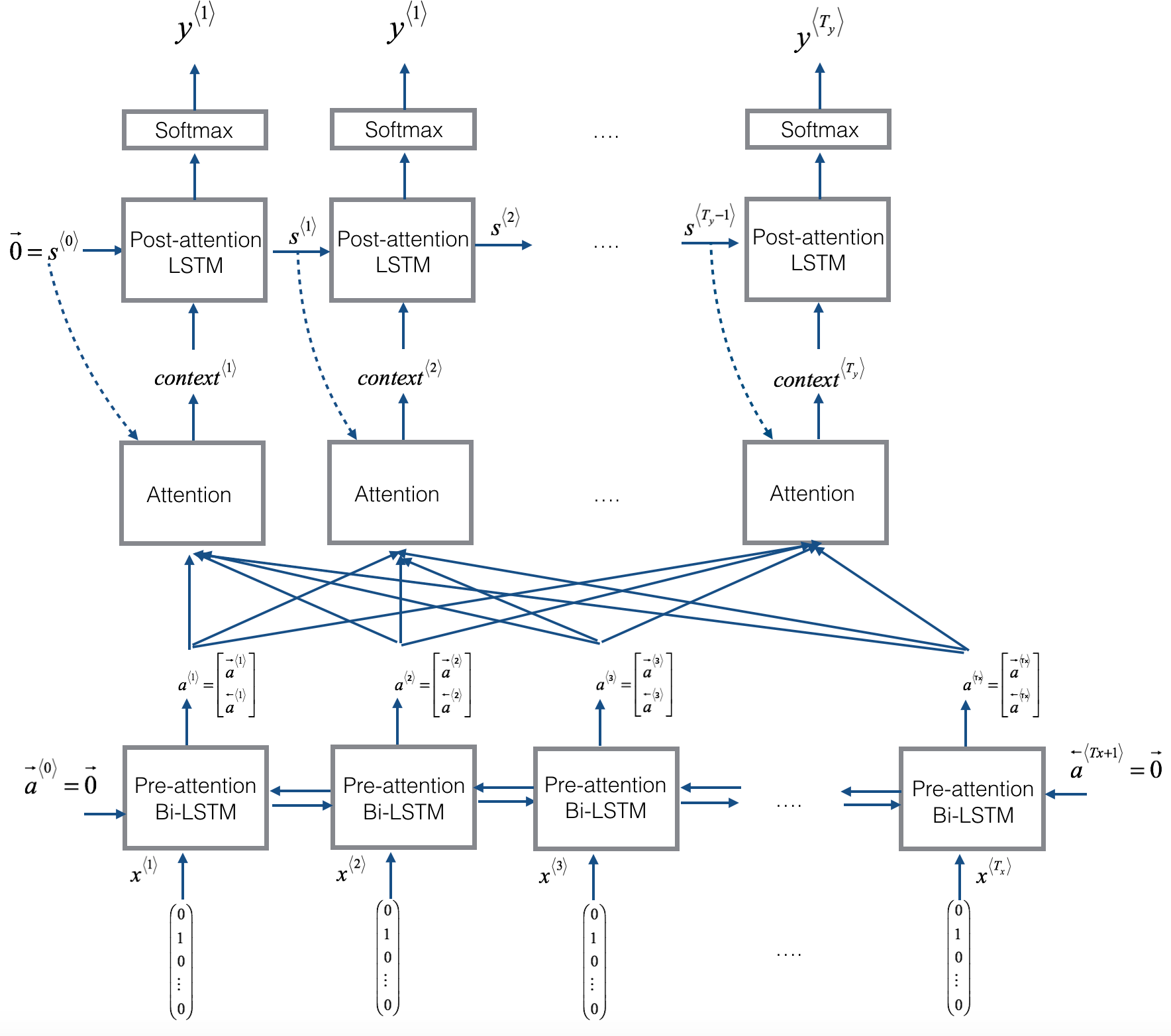
Attention model is actually split into three major parts.

First major part is a Pre-attention BRNN(you can use GRU or LSTM instead of traditional RNN here), notice that in the output we don’t have $\hat{y}^{<t>}$, we will name those outputs $a^{<t>}$, in which

such that $a^{<t>}$ is the concatenation of forward flow activation and backward flow activations.

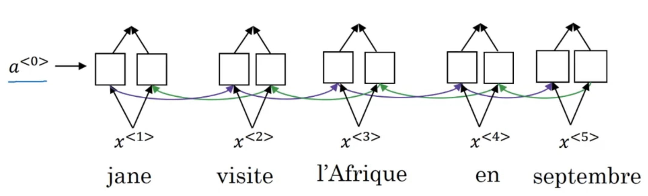
Then, using each activations $a^{<t>}$, we can compute the context for each output word, $c^{<t>}$.

The method in how we want to compute the context $c^{<t>}$ based on $a^{<t>}$ and other variables can vary, but here is an example below.

Formulas:

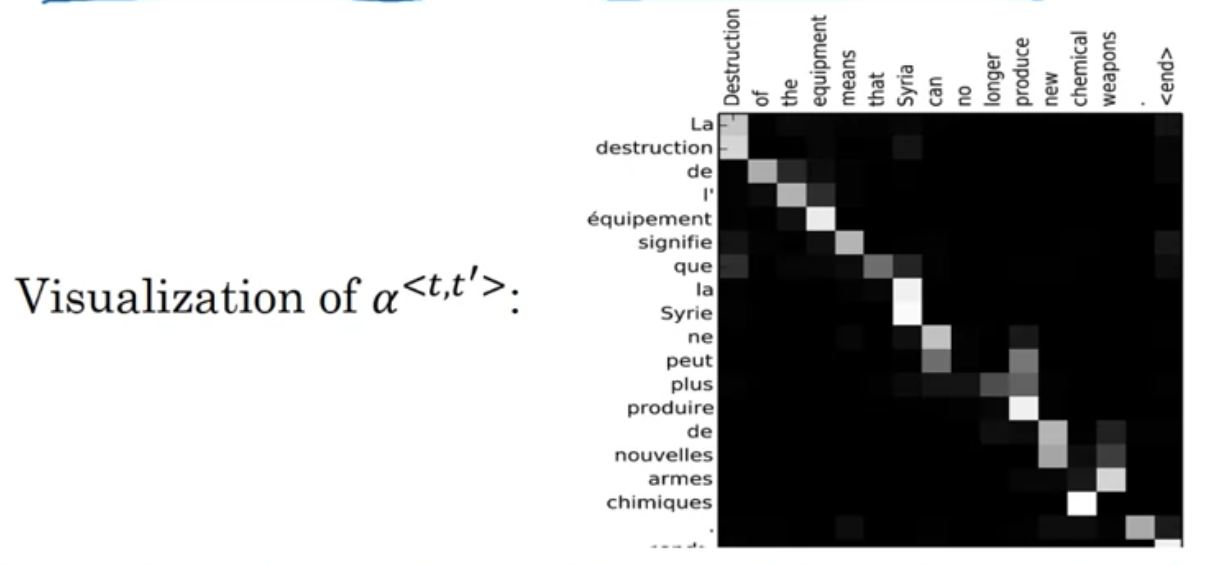
Here $\alpha^{<t,t'>}$ determines how much attention does input word $x^{<t'>}$ get when computing the output for $y^{<t>}$

$$\alpha^{<t,t'>}=\frac{exp(e^{<t,t'>})}{\sum_{k=1}^{T_x}exp(e^{t,k})} = softmax(exp(e^{<t,t'>}))$$

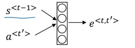
Note that below in the example context calculation below the context is calculated differently.

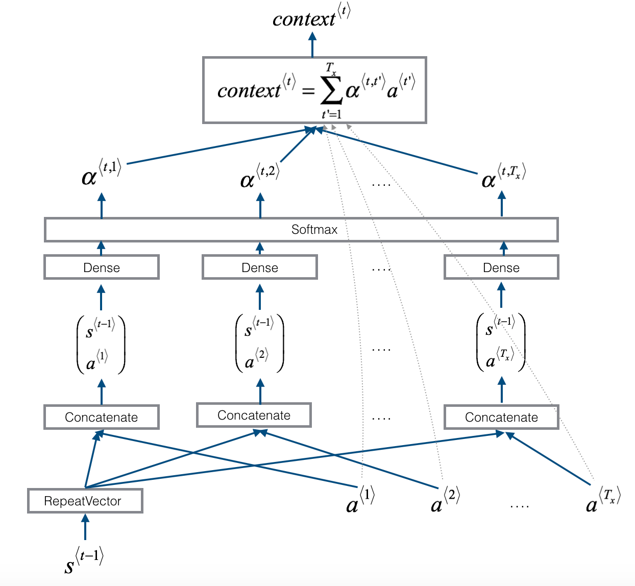
A context model example, here s^<t-1> is an activation output of our post-attention model. s^{0} = 0

Once context is computed, we can use the context $c^{<t>}$ combined with a post-attention RNN to generate the output.

Speech Recognition

Ehhh so we input lots of data into speech recognition models and it is almost always that the number of words will be less than the number of frequency input points. Plus we only need nearby sounds to know which letter or word is the person saying. So it seems like we can just do a BRNN without using the attention model.

For each output, we can output a letter or a “_”, here “_” doesn’t mean space it just means a separation of word and we will have another symbol to represent an actual space.

So we can turn “wwwww_______oo_rrrrrrrrrrrrrrrrr_____d” output and process it to be “word”.

Transformer Network

Idea: Unlike RNN, use idea from CNN + Attention

Self-Attention(”one-head”) Value

Where $q, K, V$ stands for query, key, value, respectively ⇒ sound like a database search, huh? we search through keys of inputs with a single query and whichever matches the query the best(has biggest inner product) will be put to have the most influence for its value to be in our search result.

For each input $x^{<t>}$, there is a corresponding $q^{<t>}, k^{<t>}, v^{<t>}$, and each is computed with $\vec{q}^{<t>}=W^q\vec{x}^{<t>}, \vec{k}^{<t>}=W^k\vec{x}^{<t>}, \vec{v}^{<t>}=W^v\vec{x}^{<t>}$. Where $W^q, W^k, W^v$ are learned parameter matrices.

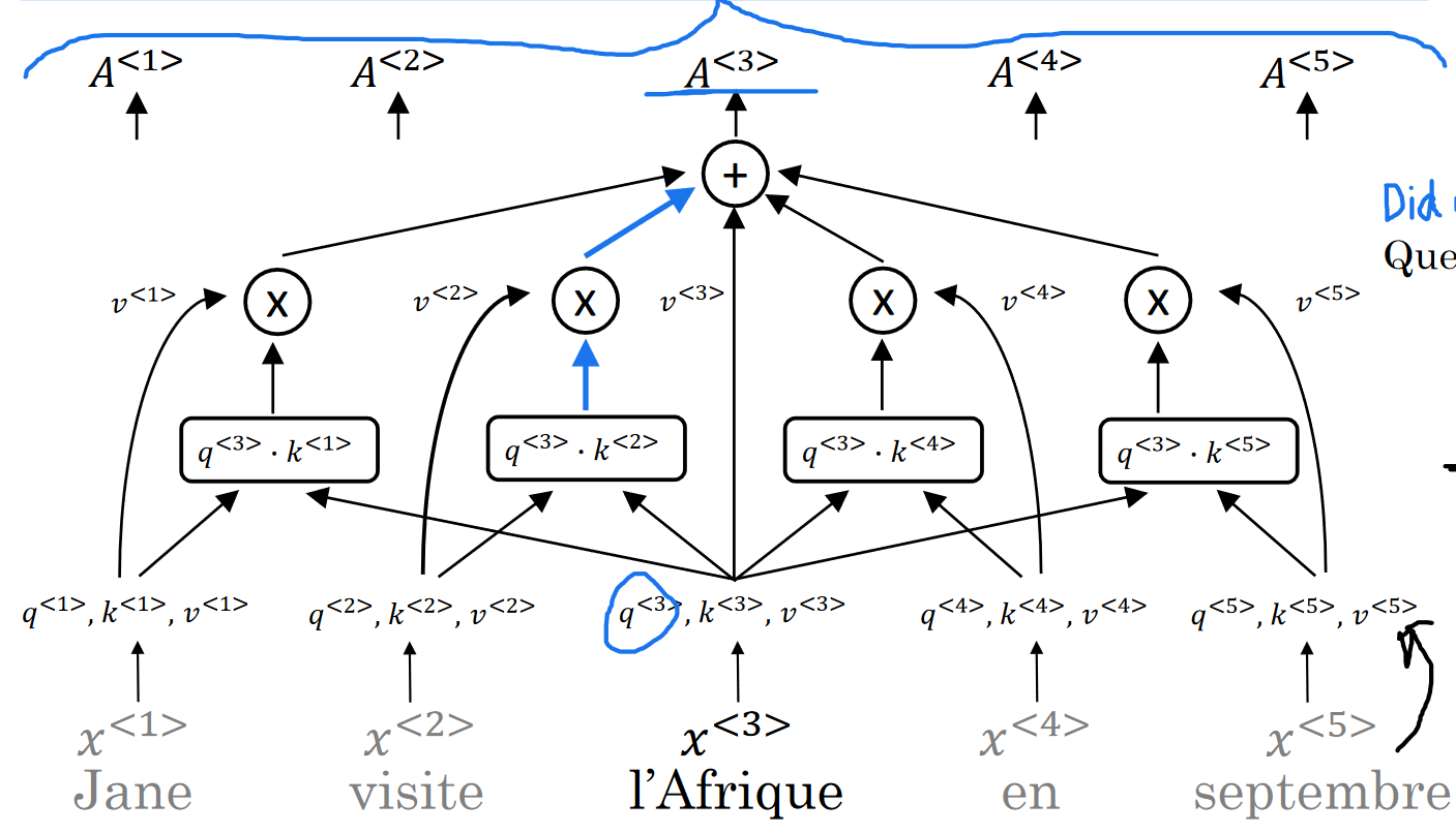
Here $d_k$ is just a scalar (dimension of k vectors) to make sure the inner product doesn’t explode.

Note: $Q = \begin{bmatrix} \vec{q}^{<1>} \cdots \vec{q}^{<T_x>} \end{bmatrix}$, and same logic for $K$ and $V$.

Multi-head Attention

It turns out that after computing QKV, instead of directly computing a one-head attention value, we can use different parameter matrices and apply them to QKV to get different sets of Q,K,Vs.

There is a hyperparameter h that determines how many heads are computed

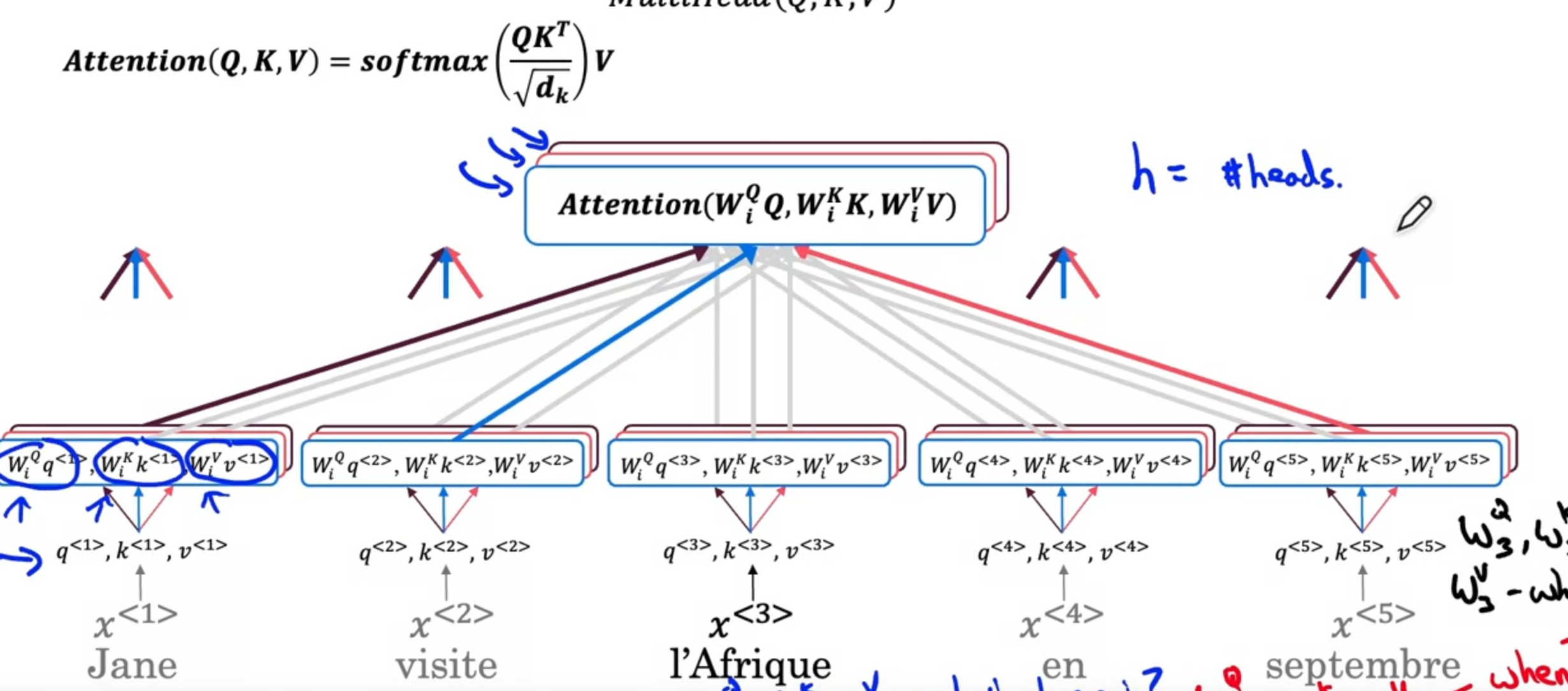
The i-th head is computed by $A(W_i^QQ,W_i^KK,W_i^VV)$, and the overall attention vector is the concatenation of all head attention vectors.

Transformer Model

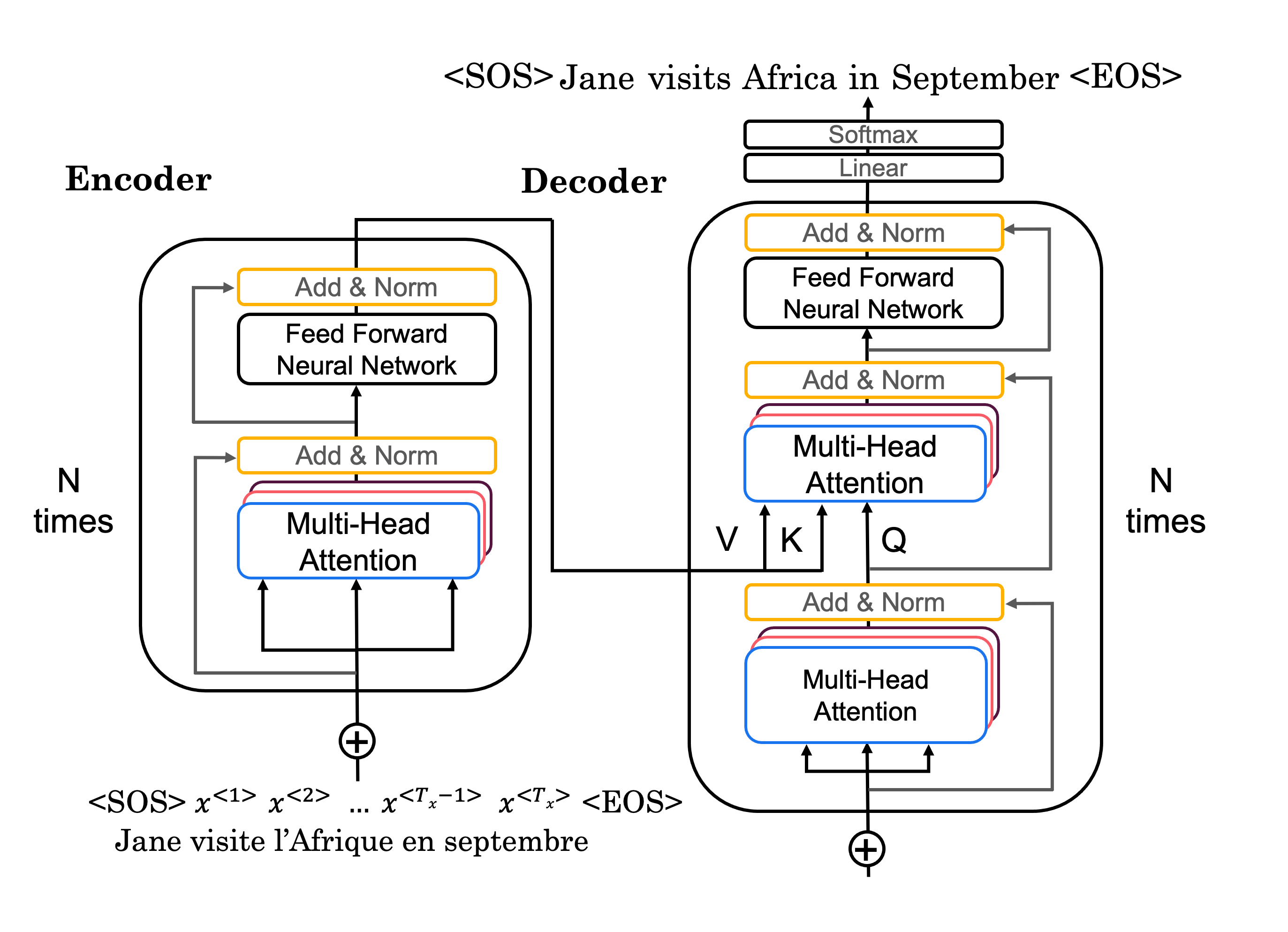
Note: The first multi-head attention in the decoder is actually a masked multi-head attention during training, because we want to pretend that all of our “predicted words” are correct while trying to train to predict the next word.

Note: Input to the decoder is the $\hat{y}^{<0>},\hat{y}^{<1>}, \dots, \hat{y}^{<t-1>}$ that has been predicted. Here $\hat{y}^{<0>} = \text{<SOS>}$. Note that this input like any other inputs to the transformer network, is limited in length, if we have n+1 words predicted while the limit is n, we would leave out the first word predicted.

Note: Add & Norm layer works like a skip layer + BatchNorm, Add basically means sum of two vectors (so that during back-prop the vanishing gradient can be less of a problem), and after summation, they will be layer-normed.

Here t denotes the position of the word in the sentence, starts with 1, and i denotes the index of the elemnt in the input vector.