Created by Yunhao Cao (Github@ToiletCommander) in Fall 2022 for UC Berkeley EECS127.
Reference Notice: Material highly and mostly derived from Prof. Ranade’s Lectures This work is licensed under a Creative Commons Attribution-NonCommercial-ShareAlike 4.0 International License
Why Optimization Control + Robotics Resource allocation problem Communications Machine Learning 🔥
Gauss used least squares technique to predict where planets would appear in the space
Optimization Forms General:
min f 0 ( x ⃗ ) subject to f i ( x ⃗ ) ≤ b i for i = 1 , 2 , … , m \min f_0(\vec{x}) \\
\text{subject to} f_i(\vec{x})\le b_i \text{ for } i=1,2,\dots,m min f 0 ( x ) subject to f i ( x ) ≤ b i for i = 1 , 2 , … , m Notation:
x ⃗ \vec{x} x x ⃗ ∈ R n \vec{x} \in \mathbb{R}^n x ∈ R n x ⃗ ∗ \vec{x}^* x ∗ x ⃗ ∈ feasible set \vec{x} \in \text{feasible set} x ∈ feasible set
Least Squares Find x ⃗ \vec{x} x A x ⃗ ≈ b ⃗ A\vec{x} \approx \vec{b} A x ≈ b ∣ ∣ A x ⃗ − b ⃗ ∣ ∣ 2 ||A\vec{x}-\vec{b}||^2 ∣∣ A x − b ∣ ∣ 2
It is relatively easy to minimize the squared norm rather than the norm because now the squared norm is differentiable and convex(any local minimum is a global minimum)
🔥
Quadratic function ⊂ Convex function \text{Quadratic function} \sub \text{Convex function} Quadratic function ⊂ Convex function
Solution:
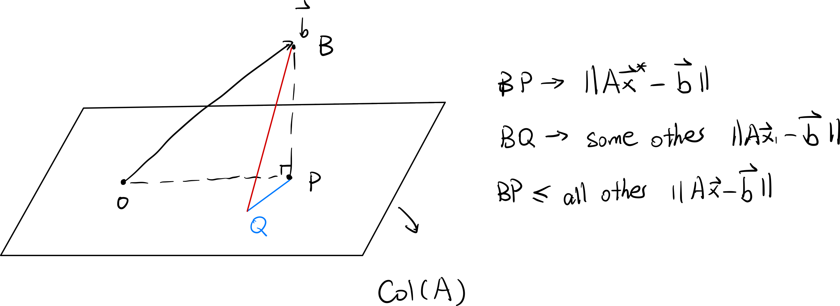
We can either derive the solution by minimizing derivative of ∣ ∣ A x ⃗ − b ∣ ∣ 2 ||A\vec{x}-b||^2 ∣∣ A x − b ∣ ∣ 2 b ⃗ \vec{b} b C o l ( A ) Col(A) C o l ( A ) A A A
Intuition of method 2 (projection) ⇒ projection of b ⃗ \vec{b} b C o l ( A ) Col(A) C o l ( A )
We derive by:
we want ( A x ⃗ − b ⃗ ) = e ⃗ where e ⃗ must be orthogonal to all of the columns of A A ⊤ e ⃗ = 0 A ⊤ ( A x ⃗ − b ⃗ ) = 0 A ⊤ A x ⃗ = A ⊤ b ⃗ x ⃗ ∗ = ( A ⊤ A ) − 1 A ⊤ b ⃗ \begin{split}
& \text{we want } (A\vec{x}- \vec{b})=\vec{e} \\
& \text{where } \vec{e} \text{ must be orthogonal to all of the columns of } A \\
& A^{\top}\vec{e}=0 \\
& A^{\top}(A\vec{x}-\vec{b})=0 \\
& A^{\top}A\vec{x}=A^{\top}\vec{b} \\
& \vec{x}^{*}=(A^\top A)^{-1} A^\top \vec{b}
\end{split} we want ( A x − b ) = e where e must be orthogonal to all of the columns of A A ⊤ e = 0 A ⊤ ( A x − b ) = 0 A ⊤ A x = A ⊤ b x ∗ = ( A ⊤ A ) − 1 A ⊤ b Linear Algebra Review Vectors, Norms, Gram-Schmidt, Fundamental Theorem of Linear Algebra
Vector x ⃗ ∈ R n \vec{x} \in \mathbb{R}^n x ∈ R n Norms If we have a vector space X X X
then a function from X → R X \rightarrow \mathbb{R} X → R
∀ x ⃗ ∈ X , ∣ ∣ x ⃗ ∣ ∣ ≥ 0 \forall \vec{x} \in X, ||\vec{x}|| \ge 0 ∀ x ∈ X , ∣∣ x ∣∣ ≥ 0 ∣ ∣ x ∣ ∣ = 0 ⟺ x ⃗ = 0 ⃗ ||x|| = 0 \iff \vec{x} = \vec{0} ∣∣ x ∣∣ = 0 ⟺ x = 0 Triangle Inequality: ∣ ∣ x ⃗ + y ⃗ ∣ ∣ ≤ ∣ ∣ x ⃗ ∣ ∣ + ∣ ∣ y ⃗ ∣ ∣ ||\vec{x} + \vec{y}|| \le ||\vec{x}|| + ||\vec{y}|| ∣∣ x + y ∣∣ ≤ ∣∣ x ∣∣ + ∣∣ y ∣∣ ∣ ∣ α x ⃗ ∣ ∣ = ∣ α ∣ × ∣ ∣ x ⃗ ∣ ∣ ||\alpha \vec{x}|| = |\alpha| \times ||\vec{x}|| ∣∣ α x ∣∣ = ∣ α ∣ × ∣∣ x ∣∣
LP Norm
∣ ∣ x ⃗ ∣ ∣ p = ( ∑ i ∣ x i ∣ p ) 1 / p , 1 ≤ p < ∞ ||\vec{x}||_p = (\sum_i |x_i|^p)^{1/p}, 1 \le p < \infin ∣∣ x ∣ ∣ p = ( i ∑ ∣ x i ∣ p ) 1/ p , 1 ≤ p < ∞ Extreme case of p → ∞ p \rightarrow \infin p → ∞
∣ ∣ x ⃗ ∣ ∣ ∞ = max i ∣ x i ∣ ||\vec{x}||_\infin = \max_{i} |x_i| ∣∣ x ∣ ∣ ∞ = i max ∣ x i ∣ TODO: Search proof for this
Intuition:
∣ ∣ x ⃗ ∣ ∣ ∞ = lim p → ∞ ( ( max i ∣ x i ∣ ) p undefined dominates + ∑ i ≠ arg max ∣ x i ∣ ∣ x i ∣ p ) 1 / p ||\vec{x}||_\infin = \lim_{p \rightarrow \infin} (\underbrace{(\max_i |x_i| )^{p}}_{\mathclap{\text{dominates}}}+\sum_{i \ne \argmax |x_i|} |x_i|^p)^{1/p} ∣∣ x ∣ ∣ ∞ = p → ∞ lim ( dominates ( i max ∣ x i ∣ ) p + i = arg max ∣ x i ∣ ∑ ∣ x i ∣ p ) 1/ p L0-Norm (Cardinality)
∣ ∣ x ⃗ ∣ ∣ 0 = ∑ i I { x i ≠ 0 } ||\vec{x}||_0 = \sum_i \mathbb{I}\{x_i \ne 0\} ∣∣ x ∣ ∣ 0 = i ∑ I { x i = 0 }
L2-Norm (Euclidean Norm)
∣ ∣ x ⃗ ∣ ∣ 2 = ∑ i x i 2 ||\vec{x}||_2 = \sqrt{\sum_i x_i^2} ∣∣ x ∣ ∣ 2 = i ∑ x i 2 Cauchy Schwartz Inequality < x ⃗ , y ⃗ > = x ⃗ ⊤ y ⃗ = ∣ ∣ x ∣ ∣ 2 × ∣ ∣ y ∣ ∣ 2 × cos θ ≤ ∣ ∣ x ∣ ∣ 2 × ∣ ∣ y ∣ ∣ 2 <\vec{x},\vec{y}>=\vec{x}^{\top}\vec{y} = ||x||_2 \times ||y||_2 \times \cos \theta \le ||x||_2 \times ||y||_2 < x , y >= x ⊤ y = ∣∣ x ∣ ∣ 2 × ∣∣ y ∣ ∣ 2 × cos θ ≤ ∣∣ x ∣ ∣ 2 × ∣∣ y ∣ ∣ 2 where θ \theta θ x ⃗ \vec{x} x y ⃗ \vec{y} y
Holder’s Inequality Generalization of Cauchy Schwartz p , q ≥ 1 , s.t. 1 p + 1 q = 1 ∣ x ⃗ t y ⃗ ∣ ≤ ∑ i ∣ x i y i ∣ ≤ ∣ ∣ x ⃗ ∣ ∣ p ∣ ∣ y ⃗ ∣ ∣ q p,q \ge 1, \text{s.t. } \frac{1}{p}+\frac{1}{q} = 1 \\
|\vec{x}^t \vec{y}| \le \sum_{i} |x_iy_i| \le ||\vec{x}||_p||\vec{y}||_q p , q ≥ 1 , s.t. p 1 + q 1 = 1 ∣ x t y ∣ ≤ i ∑ ∣ x i y i ∣ ≤ ∣∣ x ∣ ∣ p ∣∣ y ∣ ∣ q Proof not in scope for this class
First Optimization Problem max x ⃗ ⊤ y ⃗ s.t. ∣ ∣ x ⃗ ∣ ∣ p ≤ 1 , y ⃗ ∈ R n is constant \max \vec{x}^\top \vec{y} \\
\text{s.t. } ||\vec{x}||_p \le 1, \vec{y} \in \mathbb{R}^n \text{ is constant} \\
max x ⊤ y s.t. ∣∣ x ∣ ∣ p ≤ 1 , y ∈ R n is constant p=1,
x i = { sign ( y i ) if arg max i ∣ y i ∣ = i 0 otherwise x_i = \begin{cases}
\text{sign} (y_i) &\text{if } \argmax_i |y_i| = i \\
0 &\text{otherwise}
\end{cases} x i = { sign ( y i ) 0 if arg max i ∣ y i ∣ = i otherwise Produces sparse solution
max ∣ ∣ x ⃗ ∣ ∣ 1 ≤ 1 x ⃗ ⊤ y ⃗ = max i ∣ y i ∣ = ∣ ∣ y ⃗ ∣ ∣ ∞ \max_{||\vec{x}||_1 \le 1} \vec{x}^\top \vec{y} = \max_i |y_i| = ||\vec{y}||_\infin ∣∣ x ∣ ∣ 1 ≤ 1 max x ⊤ y = i max ∣ y i ∣ = ∣∣ y ∣ ∣ ∞
p = 2,
We will choose the x ⃗ \vec{x} x y ⃗ \vec{y} y cos θ \cos \theta cos θ
p = ∞ p = \infin p = ∞
x i = { 1 y i ≥ 0 − 1 y i < 0 , x ⃗ = sign ( y ⃗ ) x_i = \begin{cases}
1 &y_i \ge 0 \\
-1 &y_i < 0
\end{cases}, \\
\vec{x} = \text{sign}(\vec{y}) x i = { 1 − 1 y i ≥ 0 y i < 0 , x = sign ( y ) max ∣ ∣ x ⃗ ∣ ∣ ∞ ≤ 1 x ⃗ ⊤ y ⃗ = ∑ i ∣ y i ∣ = ∣ ∣ y ⃗ ∣ ∣ 1 \max_{||\vec{x}||_\infin \le 1} \vec{x}^\top \vec{y} = \sum_i |y_i| = ||\vec{y}||_1 ∣∣ x ∣ ∣ ∞ ≤ 1 max x ⊤ y = i ∑ ∣ y i ∣ = ∣∣ y ∣ ∣ 1 Gram-Schmidt / Orthonormalization + QR Decomposition We have a vector space X X X a 1 ⃗ , … , a n ⃗ \vec{a_1}, \dots, \vec{a_n} a 1 , … , a n
We can generate an orthonormal basis for the vector space
v 1 ⃗ = a ⃗ 1 ∣ ∣ a 1 ⃗ ∣ ∣ 2 \vec{v_1} = \frac{\vec{a}_1}{||\vec{a_1}||_2} v 1 = ∣∣ a 1 ∣ ∣ 2 a 1 v 2 ⃗ = a ⃗ 2 − p r o j v ⃗ 1 a 2 ⃗ ∣ ∣ a ⃗ 2 − p r o j v ⃗ 1 a 2 ⃗ ∣ ∣ 2 \vec{v_2}=\frac{\vec{a}_2-proj_{\vec{v}_1}{\vec{a_2}}}{||\vec{a}_2-proj_{\vec{v}_1}{\vec{a_2}}||_2} v 2 = ∣∣ a 2 − p ro j v 1 a 2 ∣ ∣ 2 a 2 − p ro j v 1 a 2 v k ⃗ = a ⃗ k − ∑ i < k p r o j v ⃗ i a ⃗ k ∣ ∣ a ⃗ k − ∑ i < k p r o j v ⃗ i a ⃗ k ∣ ∣ 2 \vec{v_k}=\frac{\vec{a}_k - \sum_{i<k} proj_{\vec{v}_i}\vec{a}_k}{||\vec{a}_k - \sum_{i<k} proj_{\vec{v}_i}\vec{a}_k||_2} v k = ∣∣ a k − ∑ i < k p ro j v i a k ∣ ∣ 2 a k − ∑ i < k p ro j v i a k where
p r o j v ⃗ t o v ⃗ f r o m = ( v ⃗ f r o m ⋅ v ⃗ ˙ t o ) v ⃗ ˙ t o = v ⃗ t o ⋅ v ⃗ f r o m ∣ ∣ v ⃗ t o ∣ ∣ 2 2 v ⃗ t o proj_{\vec{v}_{to}} \vec{v}_{from} = (\vec{v}_{from} \cdot \dot{\vec{v}}_{to}) \dot{\vec{v}}_{to} =\frac{\vec{v}_{to} \cdot \vec{v}_{from}}{||\vec{v}_{to}||_2^2} \vec{v}_{to} p ro j v t o v f ro m = ( v f ro m ⋅ v ˙ t o ) v ˙ t o = ∣∣ v t o ∣ ∣ 2 2 v t o ⋅ v f ro m v t o QR Decomposition where
A = [ a ⃗ 1 a ⃗ 2 ⋯ a ⃗ n ] A = \begin{bmatrix}
\vec{a}_1 &\vec{a}_2 &\cdots &\vec{a}_n
\end{bmatrix} A = [ a 1 a 2 ⋯ a n ] Q = [ q ⃗ 1 q 2 ⃗ ⋯ q ⃗ n ] Q = \begin{bmatrix}
\vec{q}_1 &\vec{q_2} &\cdots &\vec{q}_n
\end{bmatrix} Q = [ q 1 q 2 ⋯ q n ] R = [ r 11 r 12 ⋯ r 1 n 0 r 22 ⋯ r 2 n ⋮ 0 ⃗ ⋱ ⋮ 0 0 ⋯ r n n ] ← upper triangular matrix R = \begin{bmatrix}
r_{11} &r_{12} &\cdots &r_{1n} \\
0 &r_{22} &\cdots &r_{2n} \\
\vdots &\vec{0} &\ddots &\vdots \\
0 &0 &\cdots &r_{nn}
\end{bmatrix} \leftarrow \text{upper triangular matrix} R = ⎣ ⎡ r 11 0 ⋮ 0 r 12 r 22 0 0 ⋯ ⋯ ⋱ ⋯ r 1 n r 2 n ⋮ r nn ⎦ ⎤ ← upper triangular matrix r i j r_{ij} r ij
Fundamental Theorem of Linear Algebra A ∈ R m × n N ( A ) ⊕ undefined direct sum R ( A ⊤ ) = R n A \in \mathbb{R}^{m \times n} \\
N(A) \underbrace{\oplus}_{\mathclap{\text{direct sum}}} R(A^{\top}) = \mathbb{R}^n A ∈ R m × n N ( A ) direct sum ⊕ R ( A ⊤ ) = R n For any vector in R n \mathbb{R}^n R n We can also say:
R ( A ) ⊕ N ( A ⊤ ) = R m R(A)\oplus N(A^{\top}) = \mathbb{R}^m R ( A ) ⊕ N ( A ⊤ ) = R m To prove this, we have to use the Orthogonal Decomposition Theorem
Orthogonal Decomposition Theorem (Thm 2.1)
Let X X X S S S
∀ x ⃗ ∈ X , x ⃗ = s ⃗ + r ⃗ where s ∈ S , r ⃗ ∈ S ⊥ \forall \vec{x} \in X, \vec{x}=\vec{s}+\vec{r} \\
\text{where } s \in S, \vec{r} \in S^{\bot} ∀ x ∈ X , x = s + r where s ∈ S , r ∈ S ⊥ Note: S ⊥ = { r ⃗ ∣ ∀ s ⃗ ∈ S , < r ⃗ , s ⃗ > = 0 } S^{\bot} = \{\vec{r}|\forall \vec{s} \in S, <\vec{r},\vec{s}> = 0\} S ⊥ = { r ∣∀ s ∈ S , < r , s >= 0 } This can be summarized by
X = S ⊕ S ⊥ X = S \oplus S^{\bot} X = S ⊕ S ⊥ Proof of Orthogonal Decomposition Theorem Thanks to the ODT, now we only want to show that
N ( A ) = R ( A ⊤ ) ⊥ N(A) = R(A^{\top})^{\bot} N ( A ) = R ( A ⊤ ) ⊥ This means we need to show:
N ( A ) ⊆ R ( A ⊤ ) ⊥ R ( A ⊤ ) ⊥ ⊆ N ( A ) \begin{align}
N(A) \sube R(A^{\top})^{\bot} \\
R(A^{\top})^{\bot} \sube N(A)
\end{align}
N ( A ) ⊆ R ( A ⊤ ) ⊥ R ( A ⊤ ) ⊥ ⊆ N ( A ) To show (1)
Let x ⃗ ∈ N ( A ) \vec{x} \in N(A) x ∈ N ( A ) x ⃗ ∈ R ( A ⊤ ) ⊥ \vec{x} \in R(A^{\top})^{\bot} x ∈ R ( A ⊤ ) ⊥
∵ x ⃗ ∈ N ( A ) ∴ A x ⃗ = 0 ⃗ \because \vec{x} \in N(A) \\
\therefore A\vec{x} = \vec{0} ∵ x ∈ N ( A ) ∴ A x = 0 We want to prove:
∀ w ⃗ ∈ R ( A ⊤ ) , < x ⃗ , w ⃗ > = 0 \forall \vec{w} \in R(A^{\top}), <\vec{x},\vec{w}>=0 ∀ w ∈ R ( A ⊤ ) , < x , w >= 0 We know that since w ⃗ ∈ R ( A ⊤ ) \vec{w} \in R(A^{\top}) w ∈ R ( A ⊤ ) w ⃗ = A ⊤ y ⃗ \vec{w} = A^{\top} \vec{y} w = A ⊤ y y ⃗ \vec{y} y
< x ⃗ , w ⃗ > = < x ⃗ , A ⊤ y ⃗ > = x ⃗ ⊤ A ⊤ y ⃗ undefined it’s a sclar, so we can simply transpose it = y ⃗ ⊤ A x ⃗ = 0 <\vec{x},\vec{w}>=<\vec{x},A^{\top}\vec{y}>=\underbrace{\vec{x}^{\top}A^{\top}\vec{y}}_{\mathclap{\text{it's a sclar, so we can simply transpose it}}}=\vec{y}^{\top}A\vec{x}=0
< x , w >=< x , A ⊤ y >= it’s a sclar, so we can simply transpose it x ⊤ A ⊤ y = y ⊤ A x = 0 To show (2)
Let x ⃗ ∈ R ( A ⊤ ) ⊥ \vec{x} \in R(A^{\top})^{\bot} x ∈ R ( A ⊤ ) ⊥ x ⃗ ∈ N ( A ) \vec{x} \in N(A) x ∈ N ( A )
∵ x ⃗ ∈ R ( A ⊤ ) ⊥ ∴ ∀ w ⃗ = A ⊤ y ⃗ , where y ⃗ ∈ R m , < x ⃗ , w ⃗ > = 0 \because \vec{x} \in R(A^{\top})^{\bot} \\
\therefore \forall \vec{w} = A^{\top}\vec{y}, \text{where } \vec{y} \in \mathbb{R}^m, \\
<\vec{x},\vec{w}>=0 ∵ x ∈ R ( A ⊤ ) ⊥ ∴ ∀ w = A ⊤ y , where y ∈ R m , < x , w >= 0 < x ⃗ , A ⊤ y ⃗ > = x ⃗ ⊤ A ⊤ y ⃗ = y ⃗ ⊤ A x ⃗ = 0 , ∀ y ⃗ ∈ R n \begin{split}
<\vec{x},A^{\top}\vec{y}> &=\vec{x}^{\top}A^{\top}\vec{y} \\
&= \vec{y}^{\top}A\vec{x} = 0, \forall \vec{y} \in \mathbb{R}^n \\
\end{split} < x , A ⊤ y > = x ⊤ A ⊤ y = y ⊤ A x = 0 , ∀ y ∈ R n A specific A x ⃗ A\vec{x} A x y ⃗ ⊤ \vec{y}^{\top} y ⊤ y ⃗ \vec{y} y
Diagonalization of Matrices A = U Λ U − 1 A = U\Lambda U^{-1} A = U Λ U − 1 Not all matrices are diagonalizable
Matrices are diagonalizable when for each eigenvalue:
Algebraic Multiplicity = Geometric Multiplicity \text{Algebraic Multiplicity} = \text{Geometric Multiplicity} Algebraic Multiplicity = Geometric Multiplicity Algebraic Multiplicity:
When finding eigenvalues for a matrix we find roots of the polynomial d e t ( λ I − A ) det(\lambda I - A) d e t ( λ I − A ) λ i \lambda_i λ i λ i \lambda_i λ i
Geometric Multiplicity (for λ i \lambda_i λ i :
dim ( N ( λ i I − A ) ) \dim(N(\lambda_i I -A)) dim ( N ( λ i I − A )) 📌
Important Property:
N ( λ i I − A ) = Φ i N(\lambda_i I - A) = \Phi_i N ( λ i I − A ) = Φ i is exactly the eigen-space of
A A A corresponding to eigenvalue
λ i \lambda_i λ i Symmetric Matrices A = A ⊤ or A i j = A j i ↔ A ∈ S n A = A^{\top} \text{ or } A_{ij} = A_{ji} \leftrightarrow A \in S^n A = A ⊤ or A ij = A ji ↔ A ∈ S n e.g.
Covariance Matrices Graph Laplacians (matrix representing connectivity in a graph)
Properties:
Eigenvalues ∀ λ i , λ i ∈ R \forall \lambda_i, \lambda_i \in \mathbb{R} ∀ λ i , λ i ∈ R Eigenspaces λ i ≠ λ j \lambda_i \ne \lambda_j λ i = λ j Φ i ⊥ Φ j \Phi_i \bot \Phi_j Φ i ⊥ Φ j Φ i = N ( λ i I − A ) \Phi_i = N(\lambda_i I - A) Φ i = N ( λ i I − A ) If μ i \mu_i μ i λ i \lambda_i λ i dim ( N ( Φ i ) ) = μ i \dim(N(\Phi_i))=\mu_i dim ( N ( Φ i )) = μ i geometric and algebraic multiplicities are always equal 1-3 shows always diagnolizableA ∈ S n → A = U Λ U ⊤ A \in S^{n} \rightarrow A = U\Lambda U^{\top} A ∈ S n → A = U Λ U ⊤ where U U U Λ \Lambda Λ
Proof of Spectral Matrix has eigenvalues of the same algebraic and geometric multiplicity
Spectral Theorem Then
A = U Λ U ⊤ A = U\Lambda U^{\top} A = U Λ U ⊤ Where U U U Λ \Lambda Λ
U = [ u ⃗ 1 u ⃗ 2 ⋯ u ⃗ r undefined Range space R ( A ) u ⃗ r + 1 ⋯ u ⃗ n undefined Null Space N ( A ) ] U = \begin{bmatrix}
\underbrace{\begin{matrix}
\vec{u}_1 &\vec{u}_2 &\cdots &\vec{u}_r
\end{matrix}}_{\mathclap{\text{Range space $R(A)$}}}
&\underbrace{\begin{matrix}
\vec{u}_{r+1} &\cdots &\vec{u}_n
\end{matrix}
}_{\mathclap{\text{Null Space $N(A)$}}}
\end{bmatrix} U = [ Range space R ( A ) u 1 u 2 ⋯ u r Null Space N ( A ) u r + 1 ⋯ u n ] Λ = [ λ 1 0 ⋯ 0 0 ⋯ 0 0 λ 2 ⋯ 0 0 ⋯ 0 ⋮ ⋮ ⋱ ⋮ ⋮ ⋱ ⋮ 0 0 ⋯ λ r 0 ⋯ 0 0 0 ⋯ 0 0 ⋯ 0 ⋮ ⋮ ⋱ ⋮ ⋮ ⋱ ⋮ 0 0 ⋯ 0 0 ⋯ 0 ] \Lambda = \begin{bmatrix}
\lambda_1 &0 &\cdots &0 &0 &\cdots &0 \\
0 &\lambda_2 &\cdots &0 &0 &\cdots &0 \\
\vdots &\vdots &\ddots &\vdots &\vdots &\ddots &\vdots \\
0 &0 &\cdots &\lambda_r &0 &\cdots &0 \\
0 &0 &\cdots &0 &0 &\cdots &0\\
\vdots &\vdots &\ddots &\vdots &\vdots &\ddots &\vdots \\
0 &0 &\cdots &0 &0 &\cdots &0
\end{bmatrix} Λ = ⎣ ⎡ λ 1 0 ⋮ 0 0 ⋮ 0 0 λ 2 ⋮ 0 0 ⋮ 0 ⋯ ⋯ ⋱ ⋯ ⋯ ⋱ ⋯ 0 0 ⋮ λ r 0 ⋮ 0 0 0 ⋮ 0 0 ⋮ 0 ⋯ ⋯ ⋱ ⋯ ⋯ ⋱ ⋯ 0 0 ⋮ 0 0 ⋮ 0 ⎦ ⎤ Note: ( i < j ) ⟹ ( λ i > λ j ) (i<j) \implies (\lambda_i > \lambda_j) ( i < j ) ⟹ ( λ i > λ j ) ∀ 0 ≤ i , j ≤ r , ( λ i , v ⃗ i ) \forall 0 \le i,j \le r,(\lambda_i, \vec{v}_i) ∀0 ≤ i , j ≤ r , ( λ i , v i ) A A A
We can also write
A = ∑ i r λ i u ⃗ i u ⃗ i ⊤ \begin{split}
A &= \sum_i^r \lambda_i \vec{u}_i\vec{u}_i^{\top}
\end{split} A = i ∑ r λ i u i u i ⊤ Variational Characterization of Eigenvalues of a symmetric matrix (& Rayleigh Coefficient) Given A ∈ S n A \in S^n A ∈ S n
r ( Raylaigh Coefficient ) = x ⃗ ⊤ A x ⃗ x ⃗ ⊤ x ⃗ = x ⃗ ⊤ A x ⃗ ∣ ∣ x ⃗ ∣ ∣ 2 2 r(\text{Raylaigh Coefficient}) = \frac{\vec{x}^{\top}A\vec{x}}{\vec{x}^{\top}\vec{x}} = \frac{\vec{x}^{\top}A\vec{x}}{||\vec{x}||_2^2} r ( Raylaigh Coefficient ) = x ⊤ x x ⊤ A x = ∣∣ x ∣ ∣ 2 2 x ⊤ A x Important property:
λ min ( A ) ≤ r ≤ λ max ( A ) \lambda_{\min}(A) \le r \le \lambda_{\max}(A) λ m i n ( A ) ≤ r ≤ λ m a x ( A ) and
λ max ( A ) = max ∣ ∣ x ⃗ ∣ ∣ 2 = 1 x ⃗ ⊤ A x ⃗ λ min ( A ) = min ∣ ∣ x ⃗ ∣ ∣ 2 = 1 x ⃗ ⊤ A x ⃗ \lambda_{\max}(A) = \max_{||\vec{x}||_2=1} \vec{x}^{\top}A\vec{x} \\
\lambda_{\min}(A) = \min_{||\vec{x}||_2=1} \vec{x}^{\top}A\vec{x} λ m a x ( A ) = ∣∣ x ∣ ∣ 2 = 1 max x ⊤ A x λ m i n ( A ) = ∣∣ x ∣ ∣ 2 = 1 min x ⊤ A x Note:
x ⃗ ⊤ A x ⃗ = x ⃗ ⊤ U Λ U ⊤ x ⃗ = y ⃗ ⊤ Λ y ⃗ ( y ⃗ = U ⊤ x ⃗ ) = ∑ i = 1 r λ i y i 2 ≤ ∑ i = 1 r λ max y i 2 = λ max ∣ ∣ y ⃗ ∣ ∣ 2 2 = λ max ∣ ∣ x ⃗ ∣ ∣ 2 2 ≥ ∑ i = 1 r λ min y i 2 = λ min ∣ ∣ y ⃗ ∣ ∣ 2 2 = λ min ∣ ∣ x ⃗ ∣ ∣ 2 2 \begin{split}
\vec{x}^{\top}A\vec{x}&=\vec{x}^{\top}U\Lambda U^{\top}\vec{x} \\
&=\vec{y}^{\top}\Lambda\vec{y}\quad (\vec{y}=U^{\top}\vec{x}) \\
&=\sum_{i=1}^r \lambda_i y_i^2 \\
&\quad \le \sum_{i=1}^r \lambda_{\max} y_i^2 = \lambda_{\max}||\vec{y}||_2^2 = \lambda_{\max}||\vec{x}||_2^2 \\
&\quad \ge \sum_{i=1}^r \lambda_{\min}y_i^2=\lambda_{\min}||\vec{y}||_2^2=\lambda_{\min} ||\vec{x}||_2^2
\end{split} x ⊤ A x = x ⊤ U Λ U ⊤ x = y ⊤ Λ y ( y = U ⊤ x ) = i = 1 ∑ r λ i y i 2 ≤ i = 1 ∑ r λ m a x y i 2 = λ m a x ∣∣ y ∣ ∣ 2 2 = λ m a x ∣∣ x ∣ ∣ 2 2 ≥ i = 1 ∑ r λ m i n y i 2 = λ m i n ∣∣ y ∣ ∣ 2 2 = λ m i n ∣∣ x ∣ ∣ 2 2 Note that both U U U U ⊤ U^{\top} U ⊤
And it is obvious what what values of x ⃗ \vec{x} x
PCA + SVD Principle Component Analysis + Singular Value Decomposition 🔥
Idea: I have n-dimensional data but my data seems like they have some kind of structure in a lower dimension, how do I extract this out?
Goal of PCA:
Given data vectors x ⃗ 1 , x ⃗ 2 , … , x ⃗ n \vec{x}_1, \vec{x}_2, \dots, \vec{x}_n x 1 , x 2 , … , x n k k k w ⃗ i \vec{w}_i w i
E r r = 1 n ∑ i = 1 n e i 2 Err = \frac{1}{n}\sum_{i=1}^n e_i^2 E rr = n 1 i = 1 ∑ n e i 2 where
e i 2 = ∣ ∣ x ⃗ i − ∑ j = 1 k < w ⃗ j , x ⃗ i > w ⃗ j ∣ ∣ 2 = ∣ ∣ x ⃗ i ∣ ∣ 2 2 − ∑ j = 1 k < w ⃗ j , x ⃗ i > \begin{split}
e_i^2 &= ||\vec{x}_i - \sum_{j=1}^k <\vec{w}_j,\vec{x}_i>\vec{w}_j ||^2 \\
&= ||\vec{x}_i||_2^2 - \sum_{j=1}^k <\vec{w}_j, \vec{x}_i>
\end{split} e i 2 = ∣∣ x i − j = 1 ∑ k < w j , x i > w j ∣ ∣ 2 = ∣∣ x i ∣ ∣ 2 2 − j = 1 ∑ k < w j , x i > So our problem becomes
max { w ⃗ 1 , ⋯ , w ⃗ k } ∑ i = 1 n ∑ j = 1 k 1 n < w ⃗ j , x ⃗ i > = 1 n ∑ j = 1 k ∣ ∣ X w ⃗ j ∣ ∣ 2 = 1 n ∑ j = 1 k ( w ⃗ j ⊤ X ⊤ X undefined symmetric, use spectral theorem! w ⃗ j ) \begin{split}
\max_{\{\vec{w}_1, \cdots, \vec{w}_k\}} \sum_{i=1}^n \sum_{j=1}^k \frac{1}{n}<\vec{w}_j,\vec{x}_i>
&= \frac{1}{n}\sum_{j=1}^k||X\vec{w}_j||^2 \\
&= \frac{1}{n}\sum_{j=1}^k(\vec{w}_j^{\top}\underbrace{X^{\top}X}_{{\text{symmetric, use spectral theorem!}}}\vec{w}_j)
\end{split} { w 1 , ⋯ , w k } max i = 1 ∑ n j = 1 ∑ k n 1 < w j , x i > = n 1 j = 1 ∑ k ∣∣ X w j ∣ ∣ 2 = n 1 j = 1 ∑ k ( w j ⊤ symmetric, use spectral theorem! X ⊤ X w j )
Its easier to prove if we define data as rows so we will proceed by this…But later we can flip everything.
Data Matrix X = [ x ⃗ 1 ⊤ x ⃗ 2 ⊤ ⋮ x ⃗ n ⊤ ] \text{Data Matrix } X = \begin{bmatrix}
\vec{x}_1^{\top} \\
\vec{x}_2^{\top} \\
\vdots \\
\vec{x}_n^{\top}
\end{bmatrix} Data Matrix X = ⎣ ⎡ x 1 ⊤ x 2 ⊤ ⋮ x n ⊤ ⎦ ⎤ C = 1 n X X ⊤ = 1 n [ ∣ ∣ x ⃗ 1 ⊤ ∣ ∣ 2 < x ⃗ 1 , x ⃗ 2 > ⋯ < x ⃗ 1 , x ⃗ n > < x ⃗ 1 , x ⃗ 2 > ∣ ∣ x ⃗ 2 2 ∣ ∣ 2 ⋯ < x ⃗ 2 , x ⃗ n > ⋮ ⋮ ⋱ ⋮ < x ⃗ 1 , x ⃗ n > < x ⃗ 2 , x ⃗ n > ⋯ ∣ ∣ x ⃗ n ∣ ∣ 2 ] C = \frac{1}{n}XX^{\top}=\frac{1}{n}
\begin{bmatrix}
||\vec{x}_1^{\top}||^2 &<\vec{x}_1,\vec{x}_2> &\cdots &<\vec{x}_1,\vec{x}_n> \\
<\vec{x}_1,\vec{x}_2> &||\vec{x}_2^2||^2 &\cdots &<\vec{x}_2,\vec{x}_n> \\
\vdots &\vdots &\ddots &\vdots \\
<\vec{x}_1,\vec{x}_n> &<\vec{x}_2,\vec{x}_n> &\cdots &||\vec{x}_n||^2
\end{bmatrix} C = n 1 X X ⊤ = n 1 ⎣ ⎡ ∣∣ x 1 ⊤ ∣ ∣ 2 < x 1 , x 2 > ⋮ < x 1 , x n > < x 1 , x 2 > ∣∣ x 2 2 ∣ ∣ 2 ⋮ < x 2 , x n > ⋯ ⋯ ⋱ ⋯ < x 1 , x n > < x 2 , x n > ⋮ ∣∣ x n ∣ ∣ 2 ⎦ ⎤ Note:
X X ⊤ ∈ S n , C ∈ S n XX^{\top} \in S^n, C \in S^n X X ⊤ ∈ S n , C ∈ S n We will also define
D = 1 n X ⊤ X D = \frac{1}{n}X^{\top}X D = n 1 X ⊤ X Note that D ∈ S n D \in S^n D ∈ S n
The SVD Decomposition of A can be written as
A = U undefined m × m Σ undefined m × n V ⊤ undefined n × n A = \underbrace{U}_{m \times m} \underbrace{\Sigma}_{m \times n} \underbrace{V^{\top}}_{n \times n} A = m × m U m × n Σ n × n V ⊤ where the diagonal values of Σ \Sigma Σ A A A A ⊤ A , A A ⊤ A^{\top}A, AA^{\top} A ⊤ A , A A ⊤
The orthonormal eigenvectors of A ⊤ A A^{\top}A A ⊤ A A A A V V V Σ \Sigma Σ
The orthonormal eigenvectors of A A ⊤ AA ^{\top} A A ⊤ A A A U U U Σ \Sigma Σ
Proof of SVD Graphical Interpretation: U , V → Rotation / Reflection U, V \rightarrow \text{Rotation / Reflection} U , V → Rotation / Reflection Σ → S c a l i n g \Sigma \rightarrow Scaling Σ → S c a l in g
To understand this graphical representation of a general vector, think about decomposing the vector x ⃗ \vec{x} x V V V
x ⃗ = α 1 v ⃗ 1 + α 2 v ⃗ 2 + ⋯ + a r v ⃗ r \vec{x}=\alpha_1 \vec{v}_1 + \alpha_2 \vec{v}_2 + \cdots + a_r \vec{v}_r x = α 1 v 1 + α 2 v 2 + ⋯ + a r v r And think about how V ⊤ V^{\top} V ⊤ x ⃗ \vec{x} x A ⊤ A A^{\top}A A ⊤ A A A ⊤ AA^{\top} A A ⊤
We can write this in the compact form
A = ∑ i = 1 r σ i u ⃗ i v ⃗ i ⊤ A = \sum_{i=1}^r \sigma_i \vec{u}_i\vec{v}_i^{\top} A = i = 1 ∑ r σ i u i v i ⊤
🔥
Singular Value Decomposition is most of the time not unique because everytime we have a repeated eigenvalue (
λ i = λ j , i ≠ j \lambda_i = \lambda_j, i \ne j λ i = λ j , i = j ) then we can order the eigenbasis in different ways.
the Eckart-Young-Misky Theorem Vector Calculus f ( x ⃗ ) ∈ R n → R f(\vec{x}) \in \mathbb{R}^n \rightarrow \mathbb{R} f ( x ) ∈ R n → R Varaiya ⇒ the main theorem Scalar Calculus Review Say we have a function
f ( x ) : R → R f(x): \mathbb{R} \rightarrow \mathbb{R} f ( x ) : R → R Then the derivative
Tells the instant rate of change of f with respect to x
Taylor’s theorem Let x 0 ∈ R x_0 \in \mathbb{R} x 0 ∈ R
f ( x + Δ x ) = f ( x 0 ) + d f d x ∣ x = x 0 Δ x + 1 2 d 2 f d x 2 ∣ x = x 0 ( Δ x ) 2 + ⋯ f(x+\Delta x) = f(x_0) + \frac{df}{dx}|_{x=x_0} \Delta x + \frac{1}{2} \frac{d^2f}{dx^2} |_{x=x_0} (\Delta x)^2 + \cdots f ( x + Δ x ) = f ( x 0 ) + d x df ∣ x = x 0 Δ x + 2 1 d x 2 d 2 f ∣ x = x 0 ( Δ x ) 2 + ⋯
We usually use taylor’s theorem as an approximation tool and now if we expand our understanding of calculus onto vectors, we can make linear approximations using linear algebra!
Dimensions of Vector Gradients f ( x ⃗ ) : R n × 1 → R f(\vec{x}): \mathbb{R}^{n \times 1} \rightarrow \mathbb{R} f ( x ) : R n × 1 → R Δ x ⃗ ∈ R n × 1 \Delta \vec{x} \in \mathbb{R}^{n \times 1} Δ x ∈ R n × 1 Therefore the derivative (or the transpose of gradient)
d f d x ⃗ = ∇ f ∣ x ⃗ ⊤ ∈ R 1 × n \frac{df}{d\vec{x}} = \nabla f |_{\vec{x}}^{\top} \in \mathbb{R}^{1 \times n} d x df = ∇ f ∣ x ⊤ ∈ R 1 × n Notion of Gradient ∇ f ( x ⃗ ) \nabla f(\vec{x}) ∇ f ( x ) x ⃗ \vec{x} x
∇ f ( x ⃗ ) = [ ∂ f ∂ x 1 ∂ f ∂ x 2 ⋯ ∂ f ∂ x n ] ⊤ \nabla f(\vec{x}) = \begin{bmatrix}
\frac{\partial f}{\partial x_1} &\frac{\partial f}{\partial x_2} &\cdots &\frac{\partial f}{\partial x_n}
\end{bmatrix}^{\top} ∇ f ( x ) = [ ∂ x 1 ∂ f ∂ x 2 ∂ f ⋯ ∂ x n ∂ f ] ⊤ Notion of Hessian ∇ 2 f ( x ⃗ ) i , j = ∂ 2 f ∂ x i ∂ x j \nabla^2 f(\vec{x}) _{i,j} = \frac{\partial^2 f}{\partial x_i \partial x_j} ∇ 2 f ( x ) i , j = ∂ x i ∂ x j ∂ 2 f If we have nice smooth functions, then the order of the denominator can be interchanged. This is not generally true.
Therefore often symmetric
Jacobian Matrix Jacobian matrix describes the derivative of a vector function with respect to a vector
f ( x ⃗ ) : R n → R m f(\vec{x}): \mathbb{R}^n \rightarrow \mathbb{R}^m f ( x ) : R n → R m J = [ ∂ f ∂ x 1 ⋯ ∂ f ∂ x n ] = [ ∇ T f 1 ⋮ ∇ T f m ] = [ ∂ f 1 ∂ x 1 ⋯ ∂ f 1 ∂ x n ⋮ ⋱ ⋮ ∂ f m ∂ x 1 ⋯ ∂ f m ∂ x n ] {J} ={\begin{bmatrix}{\dfrac {\partial \mathbf {f} }{\partial x_{1}}}&\cdots &{\dfrac {\partial \mathbf {f} }{\partial x_{n}}}\end{bmatrix}}={\begin{bmatrix}\nabla ^{\mathrm {T} }f_{1}\\\vdots \\\nabla ^{\mathrm {T} }f_{m}\end{bmatrix}}={\begin{bmatrix}{\dfrac {\partial f_{1}}{\partial x_{1}}}&\cdots &{\dfrac {\partial f_{1}}{\partial x_{n}}}\\\vdots &\ddots &\vdots \\{\dfrac {\partial f_{m}}{\partial x_{1}}}&\cdots &{\dfrac {\partial f_{m}}{\partial x_{n}}}\end{bmatrix}} J = [ ∂ x 1 ∂ f ⋯ ∂ x n ∂ f ] = ⎣ ⎡ ∇ T f 1 ⋮ ∇ T f m ⎦ ⎤ = ⎣ ⎡ ∂ x 1 ∂ f 1 ⋮ ∂ x 1 ∂ f m ⋯ ⋱ ⋯ ∂ x n ∂ f 1 ⋮ ∂ x n ∂ f m ⎦ ⎤ Taylor’s Theorem for Vectors f ( x ⃗ 0 + Δ x ⃗ ) = f ( x ⃗ 0 ) + ∇ f ∣ x ⃗ = x ⃗ 0 ⊤ ( Δ x ⃗ ) + 1 2 ( Δ x ⃗ ) ⊤ ∇ 2 f ∣ x ⃗ = x ⃗ 0 undefined Hessian ( Δ x ⃗ ) + ⋯ f(\vec{x}_0+\Delta \vec{x}) = f(\vec{x}_0)+\nabla f |_{\vec{x}=\vec{x}_0}^{\top} (\Delta \vec{x}) + \frac{1}{2}(\Delta \vec{x})^{\top} \nabla^2 \underbrace{f|_{\vec{x} = \vec{x}_0}}_{\mathclap{\text{Hessian}}} (\Delta \vec{x}) + \cdots f ( x 0 + Δ x ) = f ( x 0 ) + ∇ f ∣ x = x 0 ⊤ ( Δ x ) + 2 1 ( Δ x ) ⊤ ∇ 2 Hessian f ∣ x = x 0 ( Δ x ) + ⋯ In practice you would never get higher order terms because its very hard to compute with
The main theorem f : R n → R , differentiable everywhere f: \mathbb{R}^{n} \rightarrow \mathbb{R}, \text{differentiable everywhere} f : R n → R , differentiable everywhere Then the optimization:
min f ( x ⃗ ) s.t. x ⃗ ∈ Ω \min f(\vec{x}) \\
\text{s.t. } \vec{x} \in \Omega min f ( x ) s.t. x ∈ Ω Where Ω \Omega Ω Ω ⊆ R n \Omega \sube \mathbb{R}^n Ω ⊆ R n
Then if x ⃗ ∗ \vec{x}^* x ∗
d f d x ( x ⃗ ∗ ) = 0 \frac{df}{dx}(\vec{x}^*)=0 d x df ( x ∗ ) = 0 Proof of Main’s Theorem
Optimization Forms General:
min f 0 ( x ⃗ ) subject to f i ( x ⃗ ) ≤ b i for i = 1 , 2 , … , m \min f_0(\vec{x}) \\
\text{subject to} f_i(\vec{x})\le b_i \text{ for } i=1,2,\dots,m min f 0 ( x ) subject to f i ( x ) ≤ b i for i = 1 , 2 , … , m Notation:
x ⃗ \vec{x} x x ⃗ ∈ R n \vec{x} \in \mathbb{R}^n x ∈ R n x ⃗ ∗ \vec{x}^* x ∗ x ⃗ ∈ feasible set \vec{x} \in \text{feasible set} x ∈ feasible set
Noise/Perturbation/Sensitivity Analysis A x ⃗ = y ⃗ A\vec{x}=\vec{y} A x = y y ⃗ ← y ⃗ + δ y ⃗ and because of this x ⃗ ← x ⃗ + δ x ⃗ \vec{y} \leftarrow \vec{y} +\vec{\delta_y} \text{ and because of this } \vec{x} \leftarrow \vec{x} + \vec{\delta_x} y ← y + δ y and because of this x ← x + δ x We want to measure how sensitive our solution is to a perturbation in our measurement We want to know how big is δ x ⃗ \delta \vec{x} δ x
∣ ∣ δ x ⃗ ∣ ∣ 2 ∣ ∣ x ⃗ ∣ ∣ 2 \frac{||\vec{\delta_x}||_2}{||\vec{x}||_2} ∣∣ x ∣ ∣ 2 ∣∣ δ x ∣ ∣ 2 The problem becomes:
A ( x ⃗ + δ x ⃗ ) = y ⃗ + δ y ⃗ A δ x ⃗ = δ y ⃗ δ x ⃗ = A − 1 δ y ⃗ ∣ ∣ δ x ⃗ ∣ ∣ 2 = ∣ ∣ A − 1 δ y ⃗ ∣ ∣ 2 \begin{split}
A(\vec{x}+\vec{\delta_x}) &= \vec{y} + \vec{\delta_y} \\
A\vec{\delta_x} &= \vec{\delta_y} \\
\vec{\delta_x} &= A^{-1} \vec{\delta_y} \\
||\vec{\delta_x}||_2 &= ||A^{-1} \vec{\delta_y}||_2
\end{split} A ( x + δ x ) A δ x δ x ∣∣ δ x ∣ ∣ 2 = y + δ y = δ y = A − 1 δ y = ∣∣ A − 1 δ y ∣ ∣ 2 Recall the L2 matrix norm
∣ ∣ A ∣ ∣ 2 = max ∣ ∣ y ⃗ ∣ ∣ 2 = 1 ∣ ∣ A y ⃗ ∣ ∣ 2 = max y ⃗ ∣ ∣ A y ⃗ ∣ ∣ 2 ∣ ∣ y ⃗ ∣ ∣ 2 ||A||_2 = \max_{||\vec{y}||_2 = 1} ||A\vec{y}||_2 = \max_{\vec{y}} \frac{||A\vec{y}||_2}{||\vec{y}||_2} ∣∣ A ∣ ∣ 2 = ∣∣ y ∣ ∣ 2 = 1 max ∣∣ A y ∣ ∣ 2 = y max ∣∣ y ∣ ∣ 2 ∣∣ A y ∣ ∣ 2 Also:
∣ ∣ A x ⃗ ∣ ∣ 2 = ∣ ∣ y ⃗ ∣ ∣ 2 ∣ ∣ A ∣ ∣ 2 ∣ ∣ x ⃗ ∣ ∣ 2 ≥ ∣ ∣ y ⃗ ∣ ∣ 2 ∣ ∣ x ⃗ ∣ ∣ 2 ≥ ∣ ∣ y ⃗ ∣ ∣ 2 ∣ ∣ A ∣ ∣ 2 ||A\vec{x}||_2 = ||\vec{y}||_2 \\
||A||_2 ||\vec{x}||_2 \ge ||\vec{y}||_2 \\
||\vec{x}||_2 \ge \frac{||\vec{y}||_2}{||A||_2} ∣∣ A x ∣ ∣ 2 = ∣∣ y ∣ ∣ 2 ∣∣ A ∣ ∣ 2 ∣∣ x ∣ ∣ 2 ≥ ∣∣ y ∣ ∣ 2 ∣∣ x ∣ ∣ 2 ≥ ∣∣ A ∣ ∣ 2 ∣∣ y ∣ ∣ 2
Therefore
∣ ∣ δ x ⃗ ∣ ∣ 2 = ∣ ∣ A − 1 δ y ⃗ ∣ ∣ 2 ∣ ∣ δ x ⃗ ∣ ∣ 2 ≤ ∣ ∣ A − 1 ∣ ∣ 2 ∣ ∣ δ y ⃗ ∣ ∣ 2 \begin{split}
||\vec{\delta_x}||_2 &= ||A^{-1} \vec{\delta_y}||_2 \\
||\vec{\delta_x}||_2 &\le ||A^{-1}||_2 ||\vec{\delta_y}||_2 \\
\end{split} ∣∣ δ x ∣ ∣ 2 ∣∣ δ x ∣ ∣ 2 = ∣∣ A − 1 δ y ∣ ∣ 2 ≤ ∣∣ A − 1 ∣ ∣ 2 ∣∣ δ y ∣ ∣ 2 Combining those two
∣ ∣ δ x ∣ ∣ 2 ∣ ∣ x ∣ ∣ 2 ≤ ∣ ∣ A − 1 ∣ ∣ 2 ∣ ∣ δ y ∣ ∣ 2 ∣ ∣ A ∣ ∣ 2 ∣ ∣ y ∣ ∣ 2 ∣ ∣ δ x ∣ ∣ 2 ∣ ∣ x ∣ ∣ 2 ≤ ( ∣ ∣ A ∣ ∣ 2 ) ( ∣ ∣ A − 1 ∣ ∣ 2 ) [ ∣ ∣ δ y ∣ ∣ 2 ∣ ∣ y ∣ ∣ 2 ] \begin{split}
\frac{||\delta_x||_2}{||x||_2} &\le ||A^{-1}||_2 ||\delta_y||_2 \frac{||A||_2}{||y||_2} \\
\frac{||\delta_x||_2}{||x||_2} &\le
(||A||_2)(||A^{-1}||_2) [\frac{||\delta_y||_2}{||y||_2}]
\end{split} ∣∣ x ∣ ∣ 2 ∣∣ δ x ∣ ∣ 2 ∣∣ x ∣ ∣ 2 ∣∣ δ x ∣ ∣ 2 ≤ ∣∣ A − 1 ∣ ∣ 2 ∣∣ δ y ∣ ∣ 2 ∣∣ y ∣ ∣ 2 ∣∣ A ∣ ∣ 2 ≤ ( ∣∣ A ∣ ∣ 2 ) ( ∣∣ A − 1 ∣ ∣ 2 ) [ ∣∣ y ∣ ∣ 2 ∣∣ δ y ∣ ∣ 2 ] We know that ∣ ∣ A ∣ ∣ 2 = σ m a x ( A ) ||A||_2 = \sigma_{max}(A) ∣∣ A ∣ ∣ 2 = σ ma x ( A ) ∣ ∣ A − 1 ∣ ∣ 2 = 1 / σ m i n ( A ) ||A^{-1}||_2 = 1 / \sigma_{min}(A) ∣∣ A − 1 ∣ ∣ 2 = 1/ σ min ( A )
∣ ∣ δ x ∣ ∣ 2 ∣ ∣ x ∣ ∣ 2 ≤ σ m a x ( A ) σ m i n ( A ) undefined condition number of a matrix ∣ ∣ δ y ∣ ∣ 2 ∣ ∣ y ∣ ∣ 2 \frac{||\delta_x||_2}{||x||_2} \le
\underbrace{\frac{\sigma_{max}(A)}{\sigma_{min}(A)}}_{\mathclap{\text{condition number of a matrix}}} \frac{||\delta_y||_2}{||y||_2} ∣∣ x ∣ ∣ 2 ∣∣ δ x ∣ ∣ 2 ≤ condition number of a matrix σ min ( A ) σ ma x ( A ) ∣∣ y ∣ ∣ 2 ∣∣ δ y ∣ ∣ 2 Condition Number of a matrix is σ m a x / σ m i n \sigma_{max} / \sigma_{min} σ ma x / σ min
Least Squares Find x ⃗ \vec{x} x A x ⃗ ≈ b ⃗ A\vec{x} \approx \vec{b} A x ≈ b ∣ ∣ A x ⃗ − b ⃗ ∣ ∣ 2 ||A\vec{x}-\vec{b}||^2 ∣∣ A x − b ∣ ∣ 2
It is relatively easy to minimize the squared norm rather than the norm because now the squared norm is differentiable and convex(any local minimum is a global minimum)
🔥
Quadratic function ⊂ Convex function \text{Quadratic function} \sub \text{Convex function} Quadratic function ⊂ Convex function
Solution:
We can either derive the solution by minimizing derivative of ∣ ∣ A x ⃗ − b ∣ ∣ 2 ||A\vec{x}-b||^2 ∣∣ A x − b ∣ ∣ 2 b ⃗ \vec{b} b C o l ( A ) Col(A) C o l ( A ) A A A
Intuition of method 2 (projection) ⇒ projection of b ⃗ \vec{b} b C o l ( A ) Col(A) C o l ( A )
We derive by:
we want ( A x ⃗ − b ⃗ ) = e ⃗ where e ⃗ must be orthogonal to all of the columns of A A ⊤ e ⃗ = 0 A ⊤ ( A x ⃗ − b ⃗ ) = 0 A ⊤ A x ⃗ = A ⊤ b ⃗ x ⃗ ∗ = ( A ⊤ A ) − 1 A ⊤ b ⃗ \begin{split}
& \text{we want } (A\vec{x}- \vec{b})=\vec{e} \\
& \text{where } \vec{e} \text{ must be orthogonal to all of the columns of } A \\
& A^{\top}\vec{e}=0 \\
& A^{\top}(A\vec{x}-\vec{b})=0 \\
& A^{\top}A\vec{x}=A^{\top}\vec{b} \\
& \vec{x}^{*}=(A^\top A)^{-1} A^\top \vec{b}
\end{split} we want ( A x − b ) = e where e must be orthogonal to all of the columns of A A ⊤ e = 0 A ⊤ ( A x − b ) = 0 A ⊤ A x = A ⊤ b x ∗ = ( A ⊤ A ) − 1 A ⊤ b Sensitivity analysis on least squares x ⃗ = ( A ⊤ A ) − 1 A ⊤ b ⃗ \vec{x} = (A^{\top}A)^{-1}A^\top \vec{b} x = ( A ⊤ A ) − 1 A ⊤ b rewrite:
( A ⊤ A ) x ⃗ = A ⊤ b ⃗ (A^\top A)\vec{x} = A^\top \vec{b} ( A ⊤ A ) x = A ⊤ b Look at the conditional number on A ⊤ A A^\top A A ⊤ A
Minimum Norm Problem System of equations:
A x ⃗ = b ⃗ A\vec{x} = \vec{b} A x = b where A ∈ R m × n , x ⃗ ∈ R n , b ⃗ ∈ R m A \in \mathbb{R}^{m \times n}, \vec{x} \in \mathbb{R}^n, \vec{b} \in \mathbb{R}^m A ∈ R m × n , x ∈ R n , b ∈ R m
If m ≫ n m \gg n m ≫ n
If m ≪ n m \ll n m ≪ n
One common solution for the underdetermined state is to pick the minimum energy solution
min ∣ ∣ x ⃗ ∣ ∣ 2 2 s.t. A x ⃗ = b ⃗ \min ||\vec{x}||_2^2 \\
\text{s.t. } A\vec{x}=\vec{b} min ∣∣ x ∣ ∣ 2 2 s.t. A x = b So how can we optimize this?
Components of x ⃗ \vec{x} x N ( A ) N(A) N ( A ) x ⃗ = y ⃗ + z ⃗ , y ⃗ ∈ N ( A ) , z ⃗ ∈ R ( A ⊤ ) \vec{x} = \vec{y} + \vec{z}, \vec{y} \in N(A), \vec{z} \in R(A^{\top}) x = y + z , y ∈ N ( A ) , z ∈ R ( A ⊤ ) A x ⃗ = A ( y ⃗ + z ⃗ ) = 0 + A z ⃗ = b ⃗ A\vec{x} = A(\vec{y}+\vec{z})=0+A\vec{z}=\vec{b} A x = A ( y + z ) = 0 + A z = b ∣ ∣ x ⃗ ∣ ∣ 2 2 = ∣ ∣ y ⃗ ∣ ∣ 2 2 + ∣ ∣ z ⃗ ∣ ∣ 2 2 ||\vec{x}||_2^2 = ||\vec{y}||_2^2 + ||\vec{z}||_2^2 ∣∣ x ∣ ∣ 2 2 = ∣∣ y ∣ ∣ 2 2 + ∣∣ z ∣ ∣ 2 2 So ∃ w ⃗ , z ⃗ = A ⊤ w ⃗ \exists \vec{w}, \vec{z} = A^{\top} \vec{w} ∃ w , z = A ⊤ w A z ⃗ = b ⃗ → A A ⊤ undefined If A has full rank, then this square matrix is invertible w ⃗ = b ⃗ A\vec{z}=\vec{b} \rightarrow \underbrace{A A^{\top}}_{\mathclap{\text{If $A$ has full rank, then this square matrix is invertible}}} \vec{w} = \vec{b} A z = b → If A has full rank, then this square matrix is invertible A A ⊤ w = b w ⃗ = ( A A ⊤ ) − 1 b ⃗ → z ⃗ = A ⊤ ( A A ⊤ ) − 1 b ⃗ \vec{w} = (AA^{\top})^{-1} \vec{b} \rightarrow \vec{z} = A^{\top}(AA^{\top})^{-1}\vec{b} w = ( A A ⊤ ) − 1 b → z = A ⊤ ( A A ⊤ ) − 1 b
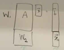
Tikhonov Regularization min x ⃗ ∣ ∣ W 1 A x ⃗ − b ⃗ ∣ ∣ 2 2 + ∣ ∣ W 2 x ⃗ − x ⃗ 0 ∣ ∣ 2 2 \min_{\vec{x}} ||W_1A\vec{x}-\vec{b}||_2^2+ ||W_2\vec{x}-\vec{x}_0||_2^2 x min ∣∣ W 1 A x − b ∣ ∣ 2 2 + ∣∣ W 2 x − x 0 ∣ ∣ 2 2 Where W 1 W_1 W 1 W 2 W_2 W 2 x ⃗ 0 \vec{x}_0 x 0
🔥
Prof. Ranade also included MAP and MLE examples of this regularization technique (and in special forms of ridge regression and MSE). See my CS189 Notes for those concepts.
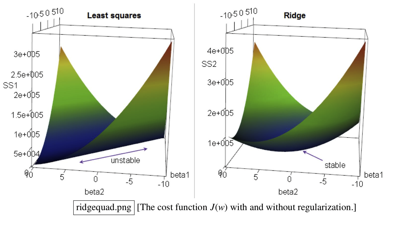
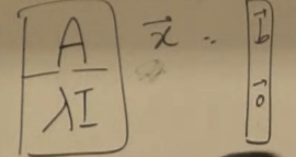
Ridge Regression Can we shift property of eigenvalues so least squares are less turbulent in response to changes in observations?
( A + λ I ) v ⃗ 1 undefined eigenvector of A = A v ⃗ 1 + λ v ⃗ 1 = λ 1 v ⃗ 1 + λ v ⃗ 1 (A+\lambda I) \underbrace{\vec{v}_1}_{\mathclap{\text{eigenvector of $A$}}} = A\vec{v}_1 + \lambda \vec{v}_1 = \lambda_1 \vec{v}_1 + \lambda \vec{v}_1 ( A + λ I ) eigenvector of A v 1 = A v 1 + λ v 1 = λ 1 v 1 + λ v 1 🧙🏽♂️
CS 189 also talks about this, basically least square + L2 Norm Mean Loss
Notation is a bit different though, CS189 uses
λ \lambda λ in the objective
f ( x ) f(x) f ( x ) while here we use
λ 2 \lambda^2 λ 2 .
Consider now the objective
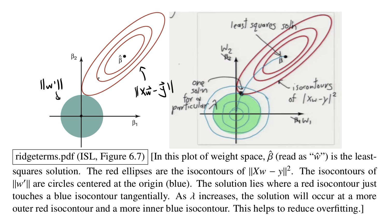
min ∣ ∣ A x ⃗ − b ⃗ ∣ ∣ 2 + λ 2 ∣ ∣ x ⃗ ∣ ∣ 2 2 \min ||A\vec{x} - \vec{b}||^2 + \lambda^2 ||\vec{x}||_2^2 min ∣∣ A x − b ∣ ∣ 2 + λ 2 ∣∣ x ∣ ∣ 2 2 Copied from prof. Schewchuk’s lecture notes Also copied from prof. Schewchuk’s slides Anther interpretation of L2 norm is we’re basically augmenting the data matrix with lambda I ∇ f ( x ⃗ ) = 2 A ⊤ A x ⃗ − 2 ( ⃗ b ⊤ A ) ⊤ + 2 λ 2 x ⃗ \nabla f(\vec{x}) = 2A^{\top}A\vec{x}- 2 \vec({b}^{\top} A)^{\top} + 2\lambda^2\vec{x} ∇ f ( x ) = 2 A ⊤ A x − 2 ( b ⊤ A ) ⊤ + 2 λ 2 x Set this gradient to 0
( A ⊤ A + λ 2 I ) x ⃗ = A ⊤ b ⃗ (A^{\top}A+\lambda^2I) \vec{x} = A^\top \vec{b} ( A ⊤ A + λ 2 I ) x = A ⊤ b So now:
x ⃗ ∗ = ( A ⊤ A + λ 2 I ) − 1 A ⊤ b ⃗ \vec{x}^* = (A^{\top}A+\lambda^2 I)^{-1}A^\top \vec{b} x ∗ = ( A ⊤ A + λ 2 I ) − 1 A ⊤ b 🔥
Also now
A ⊤ A + λ 2 I A^{\top}A + \lambda^2I A ⊤ A + λ 2 I matrix is absolutely invertible because every eigenvalue is now lower-bounded by
λ 2 \lambda^2 λ 2 If we let
x ⃗ = V z ⃗ \vec{x} = V\vec{z} x = V z And
A = U Σ V ⊤ A = U\Sigma V^\top A = U Σ V ⊤ Remember we have:
min ∣ ∣ A x ⃗ − b ⃗ ∣ ∣ 2 + λ 2 ∣ ∣ x ⃗ ∣ ∣ 2 2 = min ∣ ∣ A V z ⃗ − b ⃗ ∣ ∣ 2 + λ 2 ∣ ∣ x ⃗ ∣ ∣ 2 2 = min ∣ ∣ U Σ z ⃗ − b ⃗ ∣ ∣ 2 + λ 2 ∣ ∣ x ⃗ ∣ ∣ 2 2 \begin{split}
& \min ||A\vec{x} - \vec{b}||^2 + \lambda^2 ||\vec{x}||_2^2 \\
=& \min ||AV\vec{z}-\vec{b}||^2 + \lambda^2||\vec{x}||^2_2 \\
=& \min ||U\Sigma \vec{z} - \vec{b}||^2 + \lambda^2 ||\vec{x}||_2^2 \\
\end{split} = = min ∣∣ A x − b ∣ ∣ 2 + λ 2 ∣∣ x ∣ ∣ 2 2 min ∣∣ A V z − b ∣ ∣ 2 + λ 2 ∣∣ x ∣ ∣ 2 2 min ∣∣ U Σ z − b ∣ ∣ 2 + λ 2 ∣∣ x ∣ ∣ 2 2 Therefore
x ⃗ ∗ = V ( Σ ⊤ Σ + λ 2 I ) − 1 Σ ⊤ U ⊤ b ⃗ = V [ d i a g ( σ i σ i 2 + λ 2 ) 0 ⃗ ] U ⊤ y ⃗ \begin{split}
\vec{x}^* &= V(\Sigma^\top \Sigma+\lambda^2I)^{-1} \Sigma^\top U^\top \vec{b} \\
&=V \begin{bmatrix}
diag(\frac{\sigma_i}{\sigma_i^2 + \lambda^2}) & \vec{0}
\end{bmatrix} U^\top \vec{y}
\end{split} x ∗ = V ( Σ ⊤ Σ + λ 2 I ) − 1 Σ ⊤ U ⊤ b = V [ d ia g ( σ i 2 + λ 2 σ i ) 0 ] U ⊤ y Lasso Regression Formulation:
min x ⃗ ∣ ∣ A x ⃗ − b ⃗ ∣ ∣ 1 \min_{\vec{x}} ||A\vec{x} - \vec{b}||_1 x min ∣∣ A x − b ∣ ∣ 1 How do we solve this?
Let A x ⃗ − b ⃗ = e ⃗ A\vec{x}-\vec{b} = \vec{e} A x − b = e
then
min A x ⃗ − e ⃗ = b ⃗ ∣ ∣ e ⃗ ∣ ∣ 1 \min_{A\vec{x} - \vec{e} = \vec{b}} ||\vec{e}||_1 A x − e = b min ∣∣ e ∣ ∣ 1
Let’s consider a problem (with similar formulation)
min ∣ ∣ x ⃗ ∣ ∣ 1 s.t. A x ⃗ = b ⃗ \min ||\vec{x}||_1 \\
\text{s.t.} \\
A\vec{x} = \vec{b} min ∣∣ x ∣ ∣ 1 s.t. A x = b Not differentiable everywhere
Suppose A A A
Let x i x_i x i x i + − x i − x_i^+ - x_i^- x i + − x i − ∣ x i ∣ = x i + + x i − |x_i| = x_i^+ + x_i^- ∣ x i ∣ = x i + + x i −
Our program then becomes
min ∑ i = 1 n x i + + ∑ i = 1 n x i − A ( x ⃗ + − x ⃗ − ) = b ⃗ x i + ≥ 0 , x i − ≥ 0 \min \sum_{i=1}^n x_i^+ + \sum_{i=1}^n x_i^- \\
A(\vec{x}^+ - \vec{x}^-) = \vec{b} \\
x_i^+ \ge 0, x_i^- \ge 0 min i = 1 ∑ n x i + + i = 1 ∑ n x i − A ( x + − x − ) = b x i + ≥ 0 , x i − ≥ 0 Claim: This new program will always choose only one of x i + x_i^+ x i + or x i − x_i^- x i − nonzero
Suppose: x i + > 0 , x i − > 0 x_i^+ > 0, x_i^- > 0 x i + > 0 , x i − > 0
Consider: x i + − ϵ , x i − − ϵ x_i^+ - \epsilon, x_i^- - \epsilon x i + − ϵ , x i − − ϵ
Oops, we can strictly decrease our objective fn! ⇒ so with optimal solution, only one of x i + , x i − x_i^+, x_i^- x i + , x i −
Another problem:
min x ⃗ ∑ i = 1 n ∣ ∣ x ⃗ − b ⃗ i ∣ ∣ 1 \min_{\vec{x}} \sum_{i=1}^n ||\vec{x} - \vec{b}_i||_1 x min i = 1 ∑ n ∣∣ x − b i ∣ ∣ 1 This is solvable with a LP
Lasso Regression min x ⃗ ∣ ∣ A x ⃗ − b ⃗ ∣ ∣ 2 2 + λ ∣ ∣ x ⃗ ∣ ∣ 1 \min_{\vec{x}} ||A\vec{x}-\vec{b}||_2^2 + \lambda ||\vec{x}||_1 x min ∣∣ A x − b ∣ ∣ 2 2 + λ ∣∣ x ∣ ∣ 1 Nice property: encourages sparsity
Lasso can be reformulated as a quadratic problem
Total Least Squares What is least squares, both X X X y y y ( X + X ~ ) w ⃗ = y ⃗ + y ~ ⃗ (X+\tilde{X})\vec{w} = \vec{y} + \vec{\tilde{y}} ( X + X ~ ) w = y + y ~ We can rewrite the problem as
[ X + X ~ y ⃗ + y ~ ⃗ ] undefined Z ~ [ w ⃗ − 1 ] = 0 ⃗ \underbrace{\begin{bmatrix}
X+\tilde{X} &\vec{y}+\vec{\tilde{y}}
\end{bmatrix}}_{\mathclap{\tilde{Z}}}
\begin{bmatrix}
\vec{w} \\
-1
\end{bmatrix}
=
\vec{0} Z ~ [ X + X ~ y + y ~ ] [ w − 1 ] = 0 We know Z ~ \tilde{Z} Z ~ n n n
If we let Z = [ X y ⃗ ] Z = \begin{bmatrix} X &\vec{y} \end{bmatrix} Z = [ X y ]
Then the optimization problem becomes (an eckart-young problem)
min r k ( Z ~ ) ≤ n ∣ ∣ Z − Z ~ ∣ ∣ F \min_{rk(\tilde{Z}) \le n} ||Z - \tilde{Z}||_F r k ( Z ~ ) ≤ n min ∣∣ Z − Z ~ ∣ ∣ F Low-rank Approximation (SVD) Is there a way to store the most important parts of a matrix? ⇒ SVD? But there are multiple perspective considering parts
Matrix as an operator Matrix as a chunck of data So we can define matrix norms
“Frobenius Norm” ⇒ As a chunck of data
∣ ∣ A ∣ ∣ F = ∑ i , j A i j 2 = t r a c e ( A ⊤ A ) ||A||_F = \sqrt{\sum_{i,j} A_{ij}^2} = \sqrt{trace(A^{\top}A)} ∣∣ A ∣ ∣ F = i , j ∑ A ij 2 = t r a ce ( A ⊤ A ) 🔥
Frobenius Norms are invariant to orthonormal transforms
∣ ∣ U A ∣ ∣ F = ∣ ∣ A U ∣ ∣ F = ∣ ∣ A ∣ ∣ F ||UA||_F = ||AU||_F=||A||_F ∣∣ U A ∣ ∣ F = ∣∣ A U ∣ ∣ F = ∣∣ A ∣ ∣ F 👆TODO: Prove this as an exercise!
Frobenius Norm Invariant to Orthonormal Transform Proof
“L2-Norm / Spectral Norm” ⇒ As an operator ← max scaling of a vector
∣ ∣ A ∣ ∣ 2 = max ∣ ∣ x ⃗ ∣ ∣ 2 = 1 ∣ ∣ A x ⃗ ∣ ∣ 2 = λ m a x ( A ⊤ A ) = σ m a x ( A ) ||A||_2 = \max_{||\vec{x}||_2=1} ||A\vec{x}||_2 = \sqrt{\lambda_{max} (A^{\top}A)} = \sigma_{max} (A) ∣∣ A ∣ ∣ 2 = ∣∣ x ∣ ∣ 2 = 1 max ∣∣ A x ∣ ∣ 2 = λ ma x ( A ⊤ A ) = σ ma x ( A ) the Eckart-Young-Misky Theorem
Gradient Descent Primarily for unconstraint optimization problems p ∗ = min x ⃗ ∗ ∈ R n f 0 ( x ⃗ ) p^* = \min_{\vec{x}^* \in \mathbb{R}^n} f_0(\vec{x}) p ∗ = x ∗ ∈ R n min f 0 ( x ) We want to find p ∗ p^* p ∗ x ∗ x^* x ∗
“Guess and get better”
The best direction to improve is to use the gradient direction
x ⃗ k + 1 = x ⃗ k − η undefined step size ∇ f ( x ⃗ k ) \vec{x}_{k+1} = \vec{x}_k - \underbrace{\eta}_{\mathclap{\text{step size}}} \nabla f(\vec{x}_k) x k + 1 = x k − step size η ∇ f ( x k ) Usually SGD with constant step size is not going to converge because each data point pulls the parameters in different directions ⇒ but if we use time-dependent decreasing stepsize it’s more likely to converge Projected GD min x ⃗ ∈ X f ( x ⃗ ) \min_{\vec{x} \in X} f(\vec{x}) x ∈ X min f ( x ) Where
f ( x ) f(x) f ( x ) β \beta β So we will do the following:
x ⃗ k + 1 = Π X ( x ⃗ k − η ∇ f ( x ⃗ k ) ) \vec{x}_{k+1} = \Pi_X (\vec{x}_k - \eta \nabla f(\vec{x}_k)) x k + 1 = Π X ( x k − η ∇ f ( x k )) Where
Π X ( y ⃗ ) = arg min v ⃗ ∈ X ∣ ∣ y ⃗ − v ⃗ ∣ ∣ 2 2 \Pi_X(\vec{y}) = \argmin_{\vec{v} \in X} ||\vec{y} - \vec{v}||_2^2 Π X ( y ) = v ∈ X arg min ∣∣ y − v ∣ ∣ 2 2 Conditional GD / Frank Wolfe Let γ k \gamma_k γ k
y ⃗ k = arg min y ⃗ ∈ X ∇ f ( x ⃗ k ) ⊤ ⋅ y ⃗ \vec{y}_k = \argmin_{\vec{y} \in X} \nabla f(\vec{x}_k)^{\top} \cdot \vec{y} y k = y ∈ X arg min ∇ f ( x k ) ⊤ ⋅ y Notice here we want to find a direction that maximizes the cross-product with direction of gradient, but since we want to subtract the gradient, we can just add the direction that minimizes (maximizes negative magnitude) cross-correlation with
x ⃗ k + 1 = ( 1 − γ k ) x ⃗ k + γ k y ⃗ k = x ⃗ k + γ ( y ⃗ k − x ⃗ k ) \begin{split}
\vec{x}_{k+1} &= (1-\gamma_k) \vec{x}_k + \gamma_k \vec{y}_k \\
&=\vec{x}_k + \gamma(\vec{y}_k - \vec{x}_k)
\end{split} x k + 1 = ( 1 − γ k ) x k + γ k y k = x k + γ ( y k − x k ) Has a nice sparsity property We are basically replacing the projection with something in the set that maximizes the direction of gradient
Newton’s Method Approximate the function as a quadratic function and descend to the lowest point in the quadratic estimation f ( x ⃗ + v ⃗ ) = f ( x ⃗ ) + ∇ f ( x ⃗ ) ⊤ v ⃗ + 1 2 v ⃗ ⊤ ∇ 2 f ( x ⃗ ) v ⃗ undefined Quadratic Approximation + ⋯ f(\vec{x} + \vec{v}) = \underbrace{f(\vec{x}) + \nabla f(\vec{x})^\top \vec{v} + \frac{1}{2} \vec{v}^\top \nabla^2 f(\vec{x}) \vec{v}}_{\mathclap{\text{Quadratic Approximation}}} + \cdots f ( x + v ) = Quadratic Approximation f ( x ) + ∇ f ( x ) ⊤ v + 2 1 v ⊤ ∇ 2 f ( x ) v + ⋯ Suppose
x ⃗ 0 \vec{x}_0 x 0 General Quadratic1 2 x ⊤ H x + c ⊤ x + d \frac{1}{2} x^\top H x + c^\top x + d 2 1 x ⊤ H x + c ⊤ x + d x ∗ = − H − 1 c x^* = -H^{-1} c x ∗ = − H − 1 c Best v ⃗ \vec{v} v v ⃗ = − ( ∇ 2 f ( x ⃗ ) ) − 1 ∇ f ( x ⃗ ) \vec{v} = - (\nabla^2 f(\vec{x}))^{-1} \nabla f(\vec{x}) v = − ( ∇ 2 f ( x ) ) − 1 ∇ f ( x )
So Newton step:
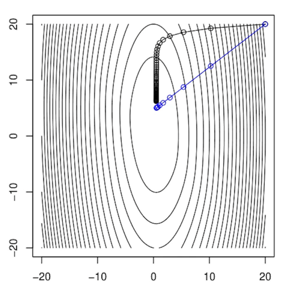
x k + 1 = x k − ( ∇ 2 f ( x ⃗ k ) ) − 1 ∇ f ( x ⃗ k ) x_{k+1} = x_k - (\nabla^2 f(\vec{x}_k))^{-1} \nabla f(\vec{x}_k) x k + 1 = x k − ( ∇ 2 f ( x k ) ) − 1 ∇ f ( x k ) If H H H
Black (Gradient Descent) vs. Blue (Newton’s Methods) Comparison to other methods:
Coordinate Descent Given an optimization objective
min x ⃗ f 0 ( x ⃗ ) \min_{\vec{x}} f_0(\vec{x}) x min f 0 ( x ) The coordinate descent will update one coordinate per timestamp, let x ⃗ ∈ R n \vec{x} \in \mathbb{R}^n x ∈ R n
( x t + 1 ) i = { arg min ( x t + 1 ) i f 0 ( x ⃗ ) if t + 1 m o d i ≡ 0 ( x t ) i otherwise (x_{t+1})_i = \begin{cases}
\argmin_{(x_{t+1})_i} f_0(\vec{x}) &\text{if } t+1 \mod i \equiv 0 \\
(x_{t})_i &\text{otherwise}
\end{cases} ( x t + 1 ) i = { arg min ( x t + 1 ) i f 0 ( x ) ( x t ) i if t + 1 mod i ≡ 0 otherwise Partitioning Problem min x ⃗ ⊤ W x ⃗ , W ∈ S n s.t. ∀ i ∈ [ 1 , n ] , x i 2 = 1 \min \vec{x}^\top W \vec{x}, W \in \mathbb{S}^n \\
\\
\text{s.t. } \forall i \in [1,n], x_i^2 = 1 min x ⊤ W x , W ∈ S n s.t. ∀ i ∈ [ 1 , n ] , x i 2 = 1 Not a convex problem ⇒ the domain is a ring
Write out the lagrangian
L ( x ⃗ , ν ⃗ ) = x ⃗ ⊤ W x ⃗ + ∑ i = 1 n ν i ( x i 2 − 1 ) = x ⃗ ⊤ W x ⃗ + x ⃗ ⊤ d i a g ( ν ⃗ ) x ⃗ − ∑ i = 1 n ν i = x ⃗ ⊤ ( W + d i a g ( ν ⃗ ) ) x ⃗ − ∑ i = 1 n ν i \begin{split}
L(\vec{x}, \vec{\nu}) &= \vec{x}^\top W \vec{x} +\sum_{i=1}^n \nu_i (x_i^2 - 1) \\
&=\vec{x}^\top W \vec{x} + \vec{x}^\top diag(\vec{\nu}) \vec{x} - \sum_{i=1}^n \nu_i \\
&=\vec{x}^\top (W+diag(\vec{\nu})) \vec{x} - \sum_{i=1}^n \nu_i \\
\end{split} L ( x , ν ) = x ⊤ W x + i = 1 ∑ n ν i ( x i 2 − 1 ) = x ⊤ W x + x ⊤ d ia g ( ν ) x − i = 1 ∑ n ν i = x ⊤ ( W + d ia g ( ν )) x − i = 1 ∑ n ν i g ( ν ⃗ ) = min x ⃗ L ( x ⃗ , ν ⃗ ) = { − ∑ i = 1 n ν i if W + d i a g ( ν ⃗ ) ≥ 0 − ∞ otherwise (choose infinitely large x ⃗ in negative eigenvalue direction) \begin{split}
g(\vec{\nu}) &= \min_{\vec{x}} L(\vec{x}, \vec{\nu}) \\
&= \begin{cases}
-\sum_{i=1}^n \nu_i &\text{if } W + diag(\vec{\nu}) \ge 0 \\
-\infin &\text{otherwise (choose infinitely large $\vec{x}$ in negative eigenvalue direction)}
\end{cases}
\end{split} g ( ν ) = x min L ( x , ν ) = { − ∑ i = 1 n ν i − ∞ if W + d ia g ( ν ) ≥ 0 otherwise (choose infinitely large x in negative eigenvalue direction) So dual problem (Semidefinite Program SDP):
max − ∑ i = 1 n ν i s.t. W + d i a g ( ν ⃗ ) ≥ 0 \max -\sum_{i=1}^n \nu_i \\
\text{s.t. } W + diag(\vec{\nu}) \ge 0 max − i = 1 ∑ n ν i s.t. W + d ia g ( ν ) ≥ 0 Solution is
ν ⃗ = λ min ( W ) → p ∗ ≥ n ⋅ λ min ( W ) \vec{\nu} = \lambda_{\min} (W) \rightarrow p^* \ge n \cdot \lambda_{\min}(W) ν = λ m i n ( W ) → p ∗ ≥ n ⋅ λ m i n ( W ) Convexity Convex Combination ∑ i = 1 n λ i x ⃗ i \sum_{i=1}^n \lambda_i \vec{x}_i ∑ i = 1 n λ i x i x ⃗ i \vec{x}_i x i λ i ≥ 0 \lambda_i \ge 0 λ i ≥ 0 ∑ i = 1 n λ i = 1 \sum_{i=1}^n \lambda_i = 1 ∑ i = 1 n λ i = 1
Convex Set Set C C C OR
Set C C C
Prove that the set of every PSD symmetric matrices are convex (4) Seperating Hyperplane Theorem If there exists two disjoint convex sets C , D C,D C , D a ⃗ ⊤ x ⃗ = b \vec{a}^\top \vec{x} = b a ⊤ x = b Proof of Seperating Hyperplane Theorem (4)
Convex Function (Bowl) f : R n → R f: \mathbb{R}^n \rightarrow \mathbb{R} f : R n → R f f f domain of f f f is a convex set and satisfies the Jensen’s Inequality:
f ( θ x ⃗ + ( 1 − θ ) y ⃗ ) ≤ θ f ( x ⃗ ) + ( 1 + θ ) f ( y ⃗ ) f(\theta \vec{x} + (1-\theta)\vec{y})\le \theta f(\vec{x})+(1+\theta)f(\vec{y}) f ( θ x + ( 1 − θ ) y ) ≤ θ f ( x ) + ( 1 + θ ) f ( y )
Epigraph :
Epi f = { ( x , t ) } , x ∈ Domain ( f ) , f ( x ) ≤ t \text{Epi }f = \{(x,t)\}, x \in \text{Domain}(f), f(x) \le t Epi f = {( x , t )} , x ∈ Domain ( f ) , f ( x ) ≤ t Property:
f f f Epi f \text{Epi }f Epi f
First-order conditions
Let the convex function f f f
Then f f f
∀ x ⃗ , y ⃗ ∈ Domain ( f ) , f ( y ⃗ ) ≥ f ( x ⃗ ) + ∇ f ( x ⃗ ) ⊤ ( y ⃗ − x ⃗ ) \forall \vec{x}, \vec{y} \in \text{Domain}(f),
f(\vec{y}) \ge f(\vec{x}) + \nabla f(\vec{x})^\top (\vec{y}-\vec{x}) ∀ x , y ∈ Domain ( f ) , f ( y ) ≥ f ( x ) + ∇ f ( x ) ⊤ ( y − x ) “Tangent line is always below the function”
If ∇ f ( x ⃗ ∗ ) = 0 \nabla f(\vec{x}^*) = 0 ∇ f ( x ∗ ) = 0 f ( y ⃗ ) ≥ f ( x ⃗ ∗ ) + 0 ( y ⃗ − x ⃗ ) f(\vec{y}) \ge f(\vec{x}^*)+0(\vec{y}-\vec{x}) f ( y ) ≥ f ( x ∗ ) + 0 ( y − x ) x ⃗ ∗ \vec{x}^* x ∗ Proof of First-order condition in convex functions (4)
Second-order conditions
Letconvex function f f f D o m ( f ) Dom(f) Do m ( f )
∇ 2 f ( x ⃗ ) ≥ 0 \nabla^2 f(\vec{x}) \ge 0 ∇ 2 f ( x ) ≥ 0 Strict Convexity Strict Convexity → Convex
D o m ( f ) Dom(f) Do m ( f )
Zero-order condition (θ ∈ ( 0 , 1 ) \theta \in (0,1) θ ∈ ( 0 , 1 )
∀ x , y ∈ D o m ( f ) , f ( θ x ⃗ + ( 1 − θ ) y ⃗ ) < θ f ( x ⃗ ) + ( 1 − θ ) f ( y ⃗ ) \forall x,y \in Dom(f), f(\theta\vec{x} + (1-\theta)\vec{y}) < \theta f(\vec{x}) + (1-\theta) f(\vec{y}) ∀ x , y ∈ Do m ( f ) , f ( θ x + ( 1 − θ ) y ) < θ f ( x ) + ( 1 − θ ) f ( y ) First-order condition:
f ( y ⃗ ) > f ( x ⃗ ) + ∇ f ( x ⃗ ) ⊤ ( y − x ) f(\vec{y}) > f(\vec{x})+\nabla f(\vec{x})^\top (y-x) f ( y ) > f ( x ) + ∇ f ( x ) ⊤ ( y − x ) Second-order condition:
∇ 2 f ( x ⃗ ) > 0 \nabla^2 f(\vec{x}) > 0 ∇ 2 f ( x ) > 0
Strong Convexity Strongly Convex → Strict Convex → Convex
f f f D o m ( f ) Dom(f) Do m ( f )
Then f f f μ \mu μ μ > 0 \mu > 0 μ > 0
∀ x ⃗ ≠ y ⃗ ∈ D o m ( f ) : f ( y ⃗ ) ≥ f ( x ⃗ ) + ∇ f ( x ⃗ ) ⊤ ( y ⃗ − x ⃗ ) + μ 2 ∣ ∣ y ⃗ − x ⃗ ∣ ∣ 2 \forall \vec{x} \ne \vec{y} \in Dom(f): \\
f(\vec{y}) \ge f(\vec{x})+\nabla f(\vec{x})^\top(\vec{y}-\vec{x})+\frac{\mu}{2}||\vec{y} - \vec{x}||^2 ∀ x = y ∈ Do m ( f ) : f ( y ) ≥ f ( x ) + ∇ f ( x ) ⊤ ( y − x ) + 2 μ ∣∣ y − x ∣ ∣ 2 Note the second-order taylor approximation:
f ( y ⃗ ) ≈ f ( x ⃗ ) + ∇ f ( x ⃗ ) ⊤ ( y ⃗ − x ⃗ ) + 1 2 ( y ⃗ − x ⃗ ) ⊤ ∇ 2 f ( x ⃗ ) ( y ⃗ − x ⃗ ) f(\vec{y}) \approx f(\vec{x}) + \nabla f(\vec{x})^\top (\vec{y}-\vec{x}) + \frac{1}{2}(\vec{y} - \vec{x})^\top \nabla^2 f(\vec{x})(\vec{y} - \vec{x}) f ( y ) ≈ f ( x ) + ∇ f ( x ) ⊤ ( y − x ) + 2 1 ( y − x ) ⊤ ∇ 2 f ( x ) ( y − x ) If we look at the term μ 2 ∣ ∣ y ⃗ − x ⃗ ∣ ∣ 2 \frac{\mu}{2} ||\vec{y} - \vec{x}||^2 2 μ ∣∣ y − x ∣ ∣ 2
1 2 ( y ⃗ − x ⃗ ) ⊤ d i a g ( μ , μ , … , μ ) ( y ⃗ − x ⃗ ) \frac{1}{2}(\vec{y}-\vec{x})^\top diag(\mu, \mu, \dots, \mu) (\vec{y}-\vec{x}) 2 1 ( y − x ) ⊤ d ia g ( μ , μ , … , μ ) ( y − x ) So we are saying that we want the hessian
∇ 2 f ( x ) ≥ μ I \nabla^2 f(x) \ge \mu I ∇ 2 f ( x ) ≥ μ I We are lower-bounding the hessian at every value L-Smooth It’s like the upper bound of “strong convexity” ⇒ strong convexity says that you can fit inside a bowl, and L-smooth says you can fit anther bowl inside your function
Convex Optimization p ∗ = min f 0 ( x ⃗ ) s.t. ∀ i ∈ [ 1 , m ] , f i ( x ⃗ ) ≤ 0 p^* = \min f_0(\vec{x}) \\
\text{s.t.} \\
\forall i\in [1,m], f_i(\vec{x}) \le 0 p ∗ = min f 0 ( x ) s.t. ∀ i ∈ [ 1 , m ] , f i ( x ) ≤ 0 Assuming f 0 ( x ⃗ ) f_0(\vec{x}) f 0 ( x ) ∀ i , f i ( x ⃗ ) \forall i, f_i(\vec{x}) ∀ i , f i ( x )
Problem Transformations Addition of “slack variables” ⇒ “epigraph” reformulationmin x ⃗ ∈ X f 0 ( x ⃗ ) → min t : f ( x ⃗ ) ≤ t , x ⃗ ∈ X t \min_{\vec{x} \in X} f_0(\vec{x}) \rightarrow \min_{t: f(\vec{x}) \le t, \vec{x} \in X} t min x ∈ X f 0 ( x ) → min t : f ( x ) ≤ t , x ∈ X t Linear Program min c ⃗ ⊤ x ⃗ s.t. A x ⃗ = b ⃗ P x ⃗ ≤ q ⃗ \min \vec{c}^\top \vec{x} \\
\text{s.t.} \\
A\vec{x} = \vec{b} \\
P\vec{x} \le \vec{q} min c ⊤ x s.t. A x = b P x ≤ q Theorem:
If min x ⃗ ∈ X c ⃗ ⊤ x ⃗ \min_{\vec{x} \in X} \vec{c}^\top \vec{x} min x ∈ X c ⊤ x X X X
x ⃗ ∗ ∈ B o u n d a r y ( X ) \vec{x}^* \in Boundary(X) x ∗ ∈ B o u n d a ry ( X ) Proof:
Assume x ⃗ ∗ \vec{x}^* x ∗ X X X r > 0 r > 0 r > 0 B a l l ∈ X Ball \in X B a ll ∈ X
∀ z ⃗ , ∣ ∣ x ⃗ − z ⃗ ∣ ∣ 2 ≤ r → z ⃗ ∈ X \forall \vec{z}, ||\vec{x} - \vec{z}||_2 \le r \rightarrow \vec{z} \in X ∀ z , ∣∣ x − z ∣ ∣ 2 ≤ r → z ∈ X Consider z ⃗ = − α c ⃗ \vec{z} = -\alpha \vec{c} z = − α c α = r ∣ ∣ c ⃗ ∣ ∣ 2 \alpha = \frac{r}{||\vec{c}||_2} α = ∣∣ c ∣ ∣ 2 r
Consider: x ⃗ ∗ + z ⃗ \vec{x}^* + \vec{z} x ∗ + z
f 0 ( x ⃗ + z ⃗ ) = c ⊤ x ⃗ ∗ − α c ⃗ ⊤ c ⃗ < f 0 ( x ⃗ ∗ ) f_0(\vec{x}+\vec{z}) = c^\top \vec{x}^* - \alpha \vec{c}^\top \vec{c} < f_0(\vec{x}^*) f 0 ( x + z ) = c ⊤ x ∗ − α c ⊤ c < f 0 ( x ∗ ) Contradiction!
Minimax Inequality With sets X , Y X, Y X , Y F F F
min x ∈ X max y ∈ Y F ( x , y ) ≥ max y ∈ Y min x ∈ X F ( x , y ) \min_{x \in X} \max_{y \in Y} F(x,y) \ge \max_{y \in Y} \min_{x \in X} F(x,y) x ∈ X min y ∈ Y max F ( x , y ) ≥ y ∈ Y max x ∈ X min F ( x , y ) Proof of Minmax Inequality (1) Lagrangian as a Dual We have optimization questions of the form
p ∗ = min f 0 ( x ⃗ ) s.t. ∀ i ∈ [ 1 , m ] , f i ( x ⃗ ) ≤ 0 ∀ i ∈ [ 1 , p ] , h i ( x ⃗ ) = 0 p^* = \min f_0(\vec{x}) \\
\\
\text{s.t.} \\
\forall i \in [1,m], f_i(\vec{x}) \le 0 \\
\forall i \in [1,p], h_i(\vec{x}) = 0
p ∗ = min f 0 ( x ) s.t. ∀ i ∈ [ 1 , m ] , f i ( x ) ≤ 0 ∀ i ∈ [ 1 , p ] , h i ( x ) = 0 Define the Lagrangian function:
L ( x ⃗ , λ ⃗ , ν ⃗ ) = f 0 ( x ⃗ ) + ∑ i = 1 m λ i f i ( x ⃗ ) + ∑ i = 1 p ν i h i ( x ⃗ ) L(\vec{x},\vec{\lambda}, \vec{\nu}) = f_0(\vec{x}) + \sum_{i=1}^m \lambda_i f_i(\vec{x}) + \sum_{i=1}^p \nu_i h_i(\vec{x}) L ( x , λ , ν ) = f 0 ( x ) + i = 1 ∑ m λ i f i ( x ) + i = 1 ∑ p ν i h i ( x ) So, the Lagrangian problem:
min x ⃗ L ( x ⃗ , λ ⃗ , ν ⃗ ) = g ( λ ⃗ , ν ⃗ ) s.t. λ ⃗ ≥ 0 \min_{\vec{x}} L(\vec{x},\vec{\lambda},\vec{\nu}) = g(\vec{\lambda},\vec{\nu}) \\
\text{s.t. } \vec{\lambda} \ge 0 x min L ( x , λ , ν ) = g ( λ , ν ) s.t. λ ≥ 0 Properties of g g g
g g g λ ⃗ , ν ⃗ \vec{\lambda}, \vec{\nu} λ , ν L ( x ⃗ , λ ⃗ , ν ⃗ ) L(\vec{x}, \vec{\lambda}, \vec{\nu}) L ( x , λ , ν ) λ ⃗ , ν ⃗ \vec{\lambda}, \vec{\nu} λ , ν Affine functions are both convex and concave What can we say about g g g Fact: pointwise max of convex function is convex Fact: pointwise min of concave function is concave g g g Because K i ( λ ⃗ , ν ⃗ ) = L ( x ⃗ i , λ ⃗ , ν ⃗ ) K_i(\vec{\lambda},\vec{\nu}) = L(\vec{x}_i, \vec{\lambda}, \vec{\nu}) K i ( λ , ν ) = L ( x i , λ , ν ) g ( λ ⃗ , ν ⃗ ) = min { ∀ i , K i ( λ , v ⃗ ) } g(\vec{\lambda}, \vec{\nu}) = \min \{\forall i, K_i(\lambda,\vec{v}) \} g ( λ , ν ) = min { ∀ i , K i ( λ , v )} Therefore g g g λ ⃗ , ν ⃗ \vec{\lambda}, \vec{\nu} λ , ν g ( λ ⃗ , ν ⃗ ) g(\vec{\lambda}, \vec{\nu}) g ( λ , ν ) p ∗ p^* p ∗ Proof of g in Lagrangian problem as a lower bound of true objective Dual problem:
max λ ⃗ ≥ 0 , ν g ( λ ⃗ , ν ⃗ ) = d ∗ → Dual Problem \max_{\vec{\lambda} \ge 0, \nu} g(\vec{\lambda}, \vec{\nu}) = d^* \rightarrow \text{Dual Problem} λ ≥ 0 , ν max g ( λ , ν ) = d ∗ → Dual Problem Maximization of a concave function with linear constraints ⇒ Convex program
Properties:
Number of variables = number of constraints of optimal Always convex problem, even if primal is not! d ∗ d^* d ∗ but it is always a lower bound d ∗ ≤ p ∗ d^* \le p^* d ∗ ≤ p ∗ Weak Duality We callp ∗ − d ∗ p^* - d^* p ∗ − d ∗ Duality Gap If p ∗ = d ∗ p^* = d^* p ∗ = d ∗ Strong Duality Sometimes hold sometimes don’t
Minmax in Lagrangian Consider
max λ ⃗ ≥ 0 , ν ⃗ L ( x ⃗ , λ ⃗ , ν ⃗ ) = max λ ⃗ ≥ 0 , ν ⃗ f 0 ( x ⃗ ) + ∑ i = 1 m λ i f i ( x ⃗ ) + ∑ i = 1 n ν i h i ( x ⃗ ) = { f 0 ( x ⃗ ) if x ⃗ is feasible ∞ \begin{split}
\max_{\vec{\lambda} \ge 0, \vec{\nu}} L(\vec{x}, \vec{\lambda}, \vec{\nu}) &= \max_{\vec{\lambda} \ge 0, \vec{\nu}} {f_0(\vec{x}) + \sum_{i=1}^m \lambda_i f_i(\vec{x}) + \sum_{i=1}^n \nu_i h_i(\vec{x})} \\
&= \begin{cases}
f_0(\vec{x}) &\text{if $\vec{x}$ is feasible} \\
\infin
\end{cases}
\end{split} λ ≥ 0 , ν max L ( x , λ , ν ) = λ ≥ 0 , ν max f 0 ( x ) + i = 1 ∑ m λ i f i ( x ) + i = 1 ∑ n ν i h i ( x ) = { f 0 ( x ) ∞ if x is feasible Note
p ∗ = min x ⃗ max λ ⃗ ≥ 0 , ν ⃗ L ( x ⃗ , λ ⃗ , ν ⃗ )
p^* = \min_{\vec{x}} \max_{\vec{\lambda} \ge 0, \vec{\nu}} L(\vec{x}, \vec{\lambda}, \vec{\nu})
p ∗ = x min λ ≥ 0 , ν max L ( x , λ , ν ) Because of minmax inequality,
Strong Duality / Slater’s Condition Strong duality holds if ∃ x 0 \exists x_0 ∃ x 0 f i ( x 0 ) < 0 ∀ i f_i(x_0) < 0 \forall i f i ( x 0 ) < 0∀ i
Refined Slater’s Condition Assume problem is convex, assume we have f 1 , f 2 , … , f k f_1, f_2, \dots, f_k f 1 , f 2 , … , f k f k + 1 , … , f m f_{k+1}, \dots, f_m f k + 1 , … , f m
Then strong duality holds if
∃ x ⃗ 0 : ∀ i ∈ [ 1 , k ] f i ( x ⃗ 0 ) ≤ 0 ∧ ∀ i ∈ [ k + 1 , m ] f i ( x ⃗ 0 ) < 0 \exists \vec{x}_0: \\
\forall i \in [1,k] f_i(\vec{x}_0) \le 0 \wedge \forall i \in [k+1,m] f_i(\vec{x}_0) < 0 ∃ x 0 : ∀ i ∈ [ 1 , k ] f i ( x 0 ) ≤ 0 ∧ ∀ i ∈ [ k + 1 , m ] f i ( x 0 ) < 0
Dual of LP Suppose the problem:
min A x ⃗ ≤ b ⃗ c ⃗ ⊤ x ⃗ \min_{A\vec{x} \le \vec{b}} \vec{c}^\top \vec{x} A x ≤ b min c ⊤ x Then
L ( x ⃗ , λ ⃗ ) = c ⃗ ⊤ x ⃗ + λ ⃗ ⊤ ( A x ⃗ − b ⃗ ) = ( A ⊤ λ ⃗ + c ⃗ ) ⊤ x ⃗ − b ⃗ ⊤ λ ⃗ L(\vec{x}, \vec{\lambda}) = \vec{c}^\top \vec{x} + \vec{\lambda}^\top(A\vec{x}-\vec{b}) = (A^\top \vec{\lambda} + \vec{c})^\top \vec{x} - \vec{b}^\top\vec{\lambda} L ( x , λ ) = c ⊤ x + λ ⊤ ( A x − b ) = ( A ⊤ λ + c ) ⊤ x − b ⊤ λ Therefore
g ( λ ⃗ ) = min x ⃗ L ( x ⃗ , λ ⃗ ) = { − ∞ if A ⊤ λ ⃗ + c ≠ 0 − b ⃗ ⊤ λ ⃗ if A ⊤ λ ⃗ + c = 0 \begin{split}
g(\vec{\lambda}) &= \min_{\vec{x}} L(\vec{x}, \vec{\lambda}) \\
&= \begin{cases}
-\infin &\text{if } A^\top \vec{\lambda}+c \ne 0 \\
-\vec{b}^\top \vec{\lambda} &\text{if } A^\top \vec{\lambda}+c = 0
\end{cases}
\end{split} g ( λ ) = x min L ( x , λ ) = { − ∞ − b ⊤ λ if A ⊤ λ + c = 0 if A ⊤ λ + c = 0 So dual is (and strong duality holds for any LP):
max λ ⃗ ≥ 0 , A ⊤ λ ⃗ + c ⃗ = 0 − b ⃗ ⊤ λ ⃗ = d ∗ \max_{\vec{\lambda} \ge 0, A^\top \vec{\lambda} + \vec{c} =0} -\vec{b}^\top \vec{\lambda} = d^* λ ≥ 0 , A ⊤ λ + c = 0 max − b ⊤ λ = d ∗ Certificate of Optimality Let ( λ ⃗ 1 , ν ⃗ 1 ) (\vec{\lambda}_1, \vec{\nu}_1) ( λ 1 , ν 1 )
We know that for any feasible point in the dual problem, the optimum of the primal function is always lower-bounded by the dual objective
p ∗ ≥ g ( λ ⃗ 1 , ν ⃗ 1 ) p^* \ge g(\vec{\lambda}_1, \vec{\nu}_1) p ∗ ≥ g ( λ 1 , ν 1 ) Then if we found a point x ⃗ 1 \vec{x}_1 x 1
f 0 ( x ⃗ 1 ) − p ∗ ≤ f 0 ( x ⃗ 1 ) − g ( λ ⃗ 1 , ν ⃗ 1 ) f_0(\vec{x}_1)-p^* \le f_0(\vec{x}_1) - g(\vec{\lambda}_1, \vec{\nu}_1) f 0 ( x 1 ) − p ∗ ≤ f 0 ( x 1 ) − g ( λ 1 , ν 1 ) So when we’ve picked a point that we know is ϵ \epsilon ϵ ϵ \epsilon ϵ
Complementary Slackness Original Problem:
p ∗ = min f 0 ( x ⃗ ) s.t. f i ( x ⃗ ) ≤ 0 ( ∀ i , 1 ≤ i ≤ m ) h i ( x ⃗ ) = 0 ( ∀ i , 1 ≤ i ≤ p ) p^* = \min f_0(\vec{x}) \\
\text{s.t.} \\
f_i(\vec{x}) \le 0 (\forall i, 1 \le i \le m) \\
h_i(\vec{x}) = 0 (\forall i, 1 \le i \le p) p ∗ = min f 0 ( x ) s.t. f i ( x ) ≤ 0 ( ∀ i , 1 ≤ i ≤ m ) h i ( x ) = 0 ( ∀ i , 1 ≤ i ≤ p ) Consider primal optimal x ⃗ ∗ \vec{x}^* x ∗ ( λ ⃗ ∗ , ν ⃗ ∗ ) (\vec{\lambda}^*, \vec{\nu}^*) ( λ ∗ , ν ∗ )
Assume strong duality holds d ∗ = g ( λ ⃗ ∗ , ν ⃗ ∗ ) = p ∗ = f 0 ( x ⃗ ∗ ) d^* = g(\vec{\lambda}^*, \vec{\nu}^*) = p^* = f_0(\vec{x}^*) d ∗ = g ( λ ∗ , ν ∗ ) = p ∗ = f 0 ( x ∗ )
Note:
g ( λ ⃗ ∗ , ν ⃗ ∗ ) = min x ⃗ ( f 0 ( x ⃗ ) + ∑ i = 1 m λ i ∗ f i ( x ⃗ ) + ∑ i = 1 p ν i ∗ h i ( x ⃗ ) ) ≤ f 0 ( x ⃗ ∗ ) + ∑ i = 1 m λ i ∗ f i ( x ⃗ ∗ ) undefined ≤ 0 + ∑ i = 1 p ν i ∗ h i ( x ⃗ ∗ ) undefined = 0 ≤ f 0 ( x ⃗ ∗ ) + 0 undefined because ( λ ⃗ ∗ , ν ⃗ ∗ ) maximizes g ( ⋯ ) + 0 \begin{split}
g(\vec{\lambda}^*, \vec{\nu}^*)
&= \min_{\vec{x}} (f_0(\vec{x}) + \sum_{i=1}^m \lambda_i^* f_i(\vec{x}) + \sum_{i=1}^p \nu_i^* h_i(\vec{x})) \\
&\le f_0(\vec{x}^*) + \underbrace{\sum_{i=1}^m \lambda_i^* f_i(\vec{x}^*)}_{\le 0} + \underbrace{\sum_{i=1}^p \nu_i^* h_i(\vec{x}^*)}_{= 0} \\
&\le f_0(\vec{x}^*) + \underbrace{0}_{\mathclap{\text{because $(\vec{\lambda}^*, \vec{\nu}^*)$ maximizes $g(\cdots)$}}} + 0
\end{split} g ( λ ∗ , ν ∗ ) = x min ( f 0 ( x ) + i = 1 ∑ m λ i ∗ f i ( x ) + i = 1 ∑ p ν i ∗ h i ( x )) ≤ f 0 ( x ∗ ) + ≤ 0 i = 1 ∑ m λ i ∗ f i ( x ∗ ) + = 0 i = 1 ∑ p ν i ∗ h i ( x ∗ ) ≤ f 0 ( x ∗ ) + because ( λ ∗ , ν ∗ ) maximizes g ( ⋯ ) 0 + 0 But in our assumption, we’ve assumed p ∗ = d ∗ p^* = d^* p ∗ = d ∗
This forces the inequality above to become equalities!
g ( λ ⃗ ∗ , ν ⃗ ∗ ) = f 0 ( x ⃗ ∗ ) + ∑ i = 1 m λ i ∗ f i ( x ⃗ ∗ ) + ∑ i = 1 p ν i ∗ h i ( x ⃗ ∗ ) = f 0 ( x ⃗ ∗ ) + 0 + 0 \begin{align}
g(\vec{\lambda}^*, \vec{\nu}^*)
&= f_0(\vec{x}^*) + \sum_{i=1}^m \lambda_i^* f_i(\vec{x}^*) + \sum_{i=1}^p \nu_i^* h_i(\vec{x}^*) \\
&= f_0(\vec{x}^*) + 0 + 0
\end{align} g ( λ ∗ , ν ∗ ) = f 0 ( x ∗ ) + i = 1 ∑ m λ i ∗ f i ( x ∗ ) + i = 1 ∑ p ν i ∗ h i ( x ∗ ) = f 0 ( x ∗ ) + 0 + 0 We’ve showed that:
min x ⃗ L ( x ⃗ , λ ⃗ ∗ , ν ⃗ ∗ ) = L ( x ⃗ ∗ , λ ⃗ ∗ , ν ⃗ ∗ ) \min_{\vec{x}} L(\vec{x},\vec{\lambda}^*,\vec{\nu}^*) = L(\vec{x}^*, \vec{\lambda}^*, \vec{\nu}^*) x min L ( x , λ ∗ , ν ∗ ) = L ( x ∗ , λ ∗ , ν ∗ ) x ⃗ ∗ \vec{x}^* x ∗ Also:
∑ i = 1 m λ i ∗ f i ( x ⃗ ∗ ) = 0 ∀ i ∈ [ 1 , m ] , λ i ∗ ⋅ f i ( x ⃗ ∗ ) = 0 \sum_{i=1}^m \lambda_i^* f_i(\vec{x}^*) = 0 \\
\forall i \in [1,m], \lambda_i^* \cdot f_i(\vec{x}^*) = 0 i = 1 ∑ m λ i ∗ f i ( x ∗ ) = 0 ∀ i ∈ [ 1 , m ] , λ i ∗ ⋅ f i ( x ∗ ) = 0 Therefore
If λ i ∗ > 0 \lambda_i^* > 0 λ i ∗ > 0 f i ( x ⃗ ∗ ) = 0 f_i(\vec{x}^*) = 0 f i ( x ∗ ) = 0 There’s a value to each extra resource If f i ( x ⃗ ∗ ) < 0 f_i(\vec{x}^*) < 0 f i ( x ∗ ) < 0 λ i ∗ = 0 \lambda_i^* = 0 λ i ∗ = 0 Condition has slack, not gonna pay money for more 👆
Those two conditions are called “complementary slackness”
Note that we did not use convexity in deriving this, only assumed strong duality.
KKT Conditions (Karush-Kuhn-Tucker Conditions) KKT Condition Part I (Necessary Conditions) Consider primal optimal x ⃗ ∗ \vec{x}^* x ∗ ( λ ⃗ ∗ , ν ⃗ ∗ ) (\vec{\lambda}^*, \vec{\nu}^*) ( λ ∗ , ν ∗ ) Assume strong duality holds d ∗ = g ( λ ⃗ ∗ , ν ⃗ ∗ ) = p ∗ = f 0 ( x ⃗ ∗ ) d^* = g(\vec{\lambda}^*, \vec{\nu}^*) = p^* = f_0(\vec{x}^*) d ∗ = g ( λ ∗ , ν ∗ ) = p ∗ = f 0 ( x ∗ ) No assumption on convexity differentiable f 0 , f i , h i f_0, f_i, h_i f 0 , f i , h i
x ⃗ ∗ , λ ⃗ ∗ , ν ⃗ ∗ \vec{x}^*, \vec{\lambda}^*, \vec{\nu}^* x ∗ , λ ∗ , ν ∗
∀ i ∈ [ 1 , m ] , f i ( x ⃗ ∗ ) ≤ 0 \forall i \in [1,m], f_i(\vec{x}^*) \le 0 ∀ i ∈ [ 1 , m ] , f i ( x ∗ ) ≤ 0 feasible set ∀ i ∈ [ 1 , p ] , h i ( x ⃗ ∗ ) = 0 \forall i \in [1,p], h_i(\vec{x}^*) = 0 ∀ i ∈ [ 1 , p ] , h i ( x ∗ ) = 0 feasible set ∀ i ∈ [ 1 , m ] , λ i ∗ ≥ 0 \forall i \in [1,m], \lambda_i^* \ge 0 ∀ i ∈ [ 1 , m ] , λ i ∗ ≥ 0 constraint on λ \lambda λ ∀ i ∈ [ 1 , m ] , λ i ∗ ⋅ f i ( x ⃗ ∗ ) = 0 \forall i \in [1,m], \lambda_i^* \cdot f_i(\vec{x}^*) = 0 ∀ i ∈ [ 1 , m ] , λ i ∗ ⋅ f i ( x ∗ ) = 0 complementary slackness ∇ f 0 ( x ⃗ ∗ ) + ∑ λ i ∗ ∇ f i ( x ⃗ ∗ ) + ∑ ν i ∗ ∇ h i ( x ⃗ ∗ ) = 0 \nabla f_0(\vec{x}^*) + \sum \lambda_i^* \nabla f_i(\vec{x}^*) + \sum \nu_i^* \nabla h_i(\vec{x}^*) = 0 ∇ f 0 ( x ∗ ) + ∑ λ i ∗ ∇ f i ( x ∗ ) + ∑ ν i ∗ ∇ h i ( x ∗ ) = 0 Gradient of lagrangian is equal to 0 We proved earlier that x ⃗ ∗ = min x ⃗ L ( x ⃗ , λ ⃗ ∗ , ν ⃗ ∗ ) \vec{x}^* = \min_{\vec{x}} L(\vec{x}, \vec{\lambda}^*, \vec{\nu}^*) x ∗ = min x L ( x , λ ∗ , ν ∗ ) implied by “the main theorem”
👆
Having those conditions do not necessarily mean that we have an optimality, but a way that we find optimal
λ ⃗ , ν ⃗ \vec{\lambda}, \vec{\nu} λ , ν is to find points where those property are met and that gives us a base space to search for optimality
KKT Condition Part II (Sufficient Condition) Convex problemsf 0 , f i f_0, f_i f 0 , f i
x ~ , λ ~ , ν ~ \tilde{x}, \tilde{\lambda}, \tilde{\nu} x ~ , λ ~ , ν ~
∀ i ∈ [ 1 , m ] , f i ( x ~ ) ≤ 0 \forall i \in [1,m], f_i(\tilde{x}) \le 0 ∀ i ∈ [ 1 , m ] , f i ( x ~ ) ≤ 0 ∀ i ∈ [ 1 , p ] , h i ( x ~ ) = 0 \forall i \in [1,p], h_i(\tilde{x}) = 0 ∀ i ∈ [ 1 , p ] , h i ( x ~ ) = 0 ∀ i ∈ [ 1 , m ] , λ ~ i ≥ 0 \forall i \in [1,m], \tilde{\lambda}_i \ge 0 ∀ i ∈ [ 1 , m ] , λ ~ i ≥ 0 ∀ i ∈ [ 1 , m ] , λ ~ i ⋅ f i ( x ~ ) = 0 \forall i \in [1,m], \tilde{\lambda}_i \cdot f_i(\tilde{x}) = 0 ∀ i ∈ [ 1 , m ] , λ ~ i ⋅ f i ( x ~ ) = 0 ∇ f 0 ( x ~ ) + ∑ λ ~ i ∇ f i ( x ~ ) + ∑ ν ~ i ∇ h i ( x ~ ) = 0 \nabla f_0(\tilde{x}) + \sum \tilde{\lambda}_i \nabla f_i(\tilde{x}) + \sum \tilde{\nu}_i \nabla h_i(\tilde{x}) = 0 ∇ f 0 ( x ~ ) + ∑ λ ~ i ∇ f i ( x ~ ) + ∑ ν ~ i ∇ h i ( x ~ ) = 0
Then:
x ~ , λ ~ , ν ~ \tilde{x}, \tilde{\lambda}, \tilde{\nu} x ~ , λ ~ , ν ~
Proof of KKT Conditions (sufficient)
Linear Program Special Case of a CONVEX optimization problem Always have strong duality Standard Form of LP min c ⃗ ⊤ x ⃗ s.t. A x ⃗ = b ⃗ x ⃗ ≥ 0 \min \vec{c}^\top \vec{x} \\
\text{s.t.} \\
A\vec{x} = \vec{b} \\
\vec{x} \ge 0 min c ⊤ x s.t. A x = b x ≥ 0 All LPs can be translated to the standard form
Eliminate inequalitiesAdd slack variables ∑ j = 1 n a i j x j ≤ b i \sum_{j=1}^n a_{ij} x_j \le b_i ∑ j = 1 n a ij x j ≤ b i ∑ i = 1 n a i j x j + s i = b i , s i ≥ 0 \sum_{i=1}^n a_{ij} x_j + s_i = b_i, s_i \ge 0 ∑ i = 1 n a ij x j + s i = b i , s i ≥ 0 Unconstrainted variablesx i ∈ R x_i \in \mathbb{R} x i ∈ R x i = x i + − x i − x_i = x_i^+ - x_i^- x i = x i + − x i − x i + ≥ 0 , x i − ≥ 0 x_i^+ \ge 0, x_i^- \ge 0 x i + ≥ 0 , x i − ≥ 0
Dual of Standard Form max − b ⃗ ⊤ λ ⃗ s.t. A ⊤ λ ⃗ + c ⃗ = 0 λ ⃗ ≥ 0 \max -\vec{b}^\top \vec{\lambda} \\
\text{s.t.} \\
A^\top \vec{\lambda} + \vec{c} = 0 \\
\vec{\lambda} \ge 0 max − b ⊤ λ s.t. A ⊤ λ + c = 0 λ ≥ 0
Simplex Algorithm Polyhedron
Set { x ⃗ ∈ R n ∣ A x ⃗ ≥ b ⃗ : A ∈ R m × n , b ⃗ ∈ R m } \{ \vec{x} \in \mathbb{R}^n | A\vec{x} \ge \vec{b} : A \in \mathbb{R}^{m \times n}, \vec{b} \in \mathbb{R}^m \} { x ∈ R n ∣ A x ≥ b : A ∈ R m × n , b ∈ R m } “Standard Form” Set { x ⃗ ∈ R l ∣ C x ⃗ = d ⃗ , x ⃗ ≥ 0 } \{ \vec{x} \in \mathbb{R}^l | C\vec{x} = \vec{d}, \vec{x} \ge 0 \} { x ∈ R l ∣ C x = d , x ≥ 0 }
Extreme Point of Polyhedron P P P
{ x ⃗ ∈ P ∣ ¬ ( ∃ y ⃗ ≠ x ⃗ , z ⃗ ≠ x ⃗ ∈ P , λ ∈ [ 0 , 1 ] : x ⃗ = λ y ⃗ + ( 1 − λ ) z ⃗ ) } \{ \vec{x} \in P | \neg(\exists \vec{y} \ne \vec{x},\vec{z} \ne \vec{x} \in P, \lambda \in [0,1] : \vec{x} = \lambda\vec{y} + (1-\lambda) \vec{z} ) \} { x ∈ P ∣¬ ( ∃ y = x , z = x ∈ P , λ ∈ [ 0 , 1 ] : x = λ y + ( 1 − λ ) z )} We cannot find two vectors for x ⃗ \vec{x} x y ⃗ \vec{y} y z ⃗ \vec{z} z
Fact:
P P P contain a line
If we assume
P P P Opt. solution exists and is finite Then:
There exists an optimal solution that is an extreme point of P P P
Proof:
P = { x ∣ A x ≤ b } , p ∗ = min x ∈ P c ⊤ x P = \{x|Ax \le b\}, p^* = \min_{x \in P} c^\top x P = { x ∣ A x ≤ b } , p ∗ = x ∈ P min c ⊤ x Let Q Q Q
Q = { x ∣ A x ≤ b , c ⊤ x = p ∗ } Q = \{x | Ax\le b, c^\top x = p^* \} Q = { x ∣ A x ≤ b , c ⊤ x = p ∗ } Q Q Q Q ⊆ P Q \sube P Q ⊆ P Q Q Q Q Q Q
If u u u Q Q Q u u u P P P
Suppose for contradiction that u u u P P P
then ∃ y , z ∈ P , y , z ≠ u \exists y, z \in P, y, z \ne u ∃ y , z ∈ P , y , z = u λ y + ( 1 − λ ) z = u , λ ∈ ( 0 , 1 ) \lambda y + (1-\lambda) z = u, \lambda \in (0,1) λ y + ( 1 − λ ) z = u , λ ∈ ( 0 , 1 )
We know c ⊤ u = p ∗ c^\top u = p^* c ⊤ u = p ∗ λ c ⊤ y + ( 1 − λ ) c ⊤ z = c ⊤ u = p ∗ \lambda c^\top y + (1-\lambda) c^\top z = c^\top u = p^* λ c ⊤ y + ( 1 − λ ) c ⊤ z = c ⊤ u = p ∗
We know since p ∗ p^* p ∗
c ⊤ y ≥ p ∗ , c ⊤ z ≥ p ∗ c^\top y \ge p^*, c^\top z \ge p^* c ⊤ y ≥ p ∗ , c ⊤ z ≥ p ∗ By the above strict equation, we infer
c ⊤ y = c ⊤ z = p ∗ c^\top y = c^\top z = p^* c ⊤ y = c ⊤ z = p ∗ So now y , z ∈ Q y, z \in Q y , z ∈ Q
But u u u Q Q Q
Therefore u u u P P P
Quadratic Programs min 1 2 x ⃗ ⊤ H x ⃗ + c ⃗ ⊤ x ⃗ s.t. A x ⃗ ≤ b ⃗ C x ⃗ = d ⃗ \min \frac{1}{2} \vec{x}^\top H \vec{x} + \vec{c}^\top \vec{x} \\
\text{s.t.} \\
A\vec{x} \le \vec{b} \\
C\vec{x} = \vec{d} min 2 1 x ⊤ H x + c ⊤ x s.t. A x ≤ b C x = d If H ∈ S n H \in \mathbb{S}^n H ∈ S n H ≥ 0 H \ge 0 H ≥ 0
Eigenvalues of H ∈ S n H \in \mathbb{S}^n H ∈ S n
H H H p ∗ = − ∞ p^* = -\infin p ∗ = − ∞ H ≥ 0 H \ge 0 H ≥ 0 c ⃗ ∈ R ( H ) \vec{c} \in R(H) c ∈ R ( H ) Rewrite f ( x ⃗ ) = 1 2 ( x ⃗ − x ⃗ 0 ) ⊤ H ( x ⃗ − x ⃗ 0 ) + α f(\vec{x}) = \frac{1}{2} (\vec{x} - \vec{x}_0)^\top H (\vec{x} - \vec{x}_0) + \alpha f ( x ) = 2 1 ( x − x 0 ) ⊤ H ( x − x 0 ) + α α \alpha α If H H H x ⃗ ∗ = − H − 1 c ⃗ \vec{x}^* = - H^{-1} \vec{c} x ∗ = − H − 1 c If not (H H H − H x ⃗ 0 = c ⃗ -H \vec{x}_0 = \vec{c} − H x 0 = c H † = U Σ − 1 V ⊤ H^{\dagger} = U\Sigma^{-1}V^\top H † = U Σ − 1 V ⊤ H ≥ 0 , c ⃗ ∉ R ( H ) H \ge 0, \vec{c} \notin R(H) H ≥ 0 , c ∈ / R ( H ) c ⃗ = − H x ⃗ 0 + r ⃗ \vec{c} = -H \vec{x}_0 + \vec{r} c = − H x 0 + r f ( r ⃗ ) = 1 2 r ⃗ ⊤ H r ⃗ + c ⃗ ⊤ r ⃗ = ∣ ∣ r ⃗ ∣ ∣ 2 2 f(\vec{r}) = \frac{1}{2} \vec{r}^\top H \vec{r} + \vec{c}^\top \vec{r} = ||\vec{r}||_2^2 f ( r ) = 2 1 r ⊤ H r + c ⊤ r = ∣∣ r ∣ ∣ 2 2
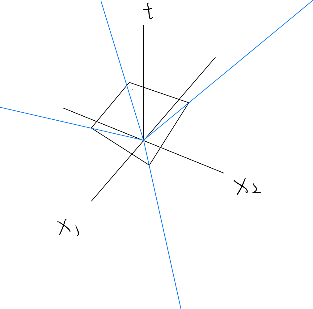
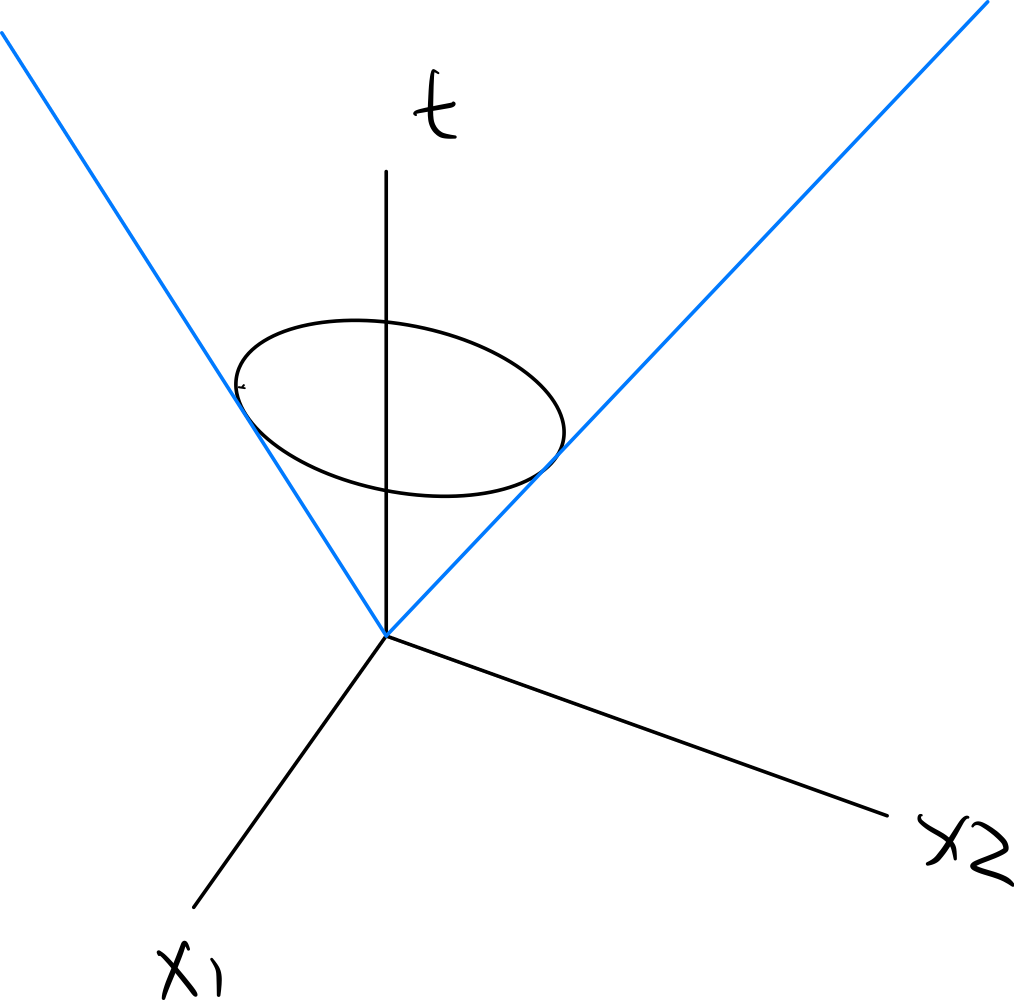
Cones Cone: Set of points C ⊆ R n C \sube \mathbb{R}^n C ⊆ R n ∀ x ⃗ ∈ C , ∀ α ≥ 0 , α x ⃗ ∈ C \forall \vec{x} \in C, \forall \alpha \ge 0, \alpha \vec{x} \in C ∀ x ∈ C , ∀ α ≥ 0 , α x ∈ C
Convex ConeA cone C C C ∀ θ 1 , θ 2 ≥ 0 , θ 1 x ⃗ 1 + θ 2 x ⃗ 2 ∈ C \forall \theta_1, \theta_2 \ge 0, \theta_1 \vec{x}_1 + \theta_2 \vec{x}_2 \in C ∀ θ 1 , θ 2 ≥ 0 , θ 1 x 1 + θ 2 x 2 ∈ C Polyhedral ConeC = { ( x ⃗ , t ) ∣ A x ⃗ ≤ b ⃗ t , t ∈ R , t ≥ 0 } C = \{ (\vec{x},t) | A\vec{x} \le \vec{b}t, t \in \mathbb{R}, t \ge 0 \} C = {( x , t ) ∣ A x ≤ b t , t ∈ R , t ≥ 0 } Polyhedral Cone Ellipsoidal ConeEquation for Ellipsex ⊤ P x + q ⊤ x + r ≤ 0 , P > 0 x^\top P x + q^\top x + r \le 0, P > 0 x ⊤ P x + q ⊤ x + r ≤ 0 , P > 0 ∣ ∣ A x + b ∣ ∣ 2 2 ≤ c 2 ||Ax+b||_2^2 \le c^2 ∣∣ A x + b ∣ ∣ 2 2 ≤ c 2 x ⊤ A ⊤ A x + 2 b ⊤ A x + b ⊤ b − c 2 ≤ 0 x^\top A^\top A x + 2 b^\top A x + b^\top b -c^2 \le 0 x ⊤ A ⊤ A x + 2 b ⊤ A x + b ⊤ b − c 2 ≤ 0 Ellipsoidal Cone EquationC = { ( x , t ) ; ∣ ∣ A x + b t ∣ ∣ 2 ≤ c t } C = \{ (x,t) ; ||Ax + bt||_2 \le ct \} C = {( x , t ) ; ∣∣ A x + b t ∣ ∣ 2 ≤ c t } ( α x , α t ) ∈ C , ∀ α ≥ 0 , ( x , t ) ∈ C (\alpha x, \alpha t) \in C, \forall \alpha \ge 0, (x,t) \in C ( αx , α t ) ∈ C , ∀ α ≥ 0 , ( x , t ) ∈ C Special Case:Second-Order ConeC ⊂ R n + 1 , C = { ( x ⃗ , t ) ; ∣ ∣ x ⃗ ∣ ∣ 2 ≤ t } C \sub \mathbb{R}^{n+1}, C = \{ (\vec{x}, t) ; ||\vec{x}||_2 \le t \} C ⊂ R n + 1 , C = {( x , t ) ; ∣∣ x ∣ ∣ 2 ≤ t } Second-order Cone in R 3 \mathbb{R}^3 R 3
Second Order Cone Program min q ⃗ ⊤ x ⃗ s.t. ∀ i ∈ { 1 , … , m } , ∣ ∣ A i x ⃗ + b ⃗ i ∣ ∣ 2 ≤ c ⃗ i ⊤ x ⃗ + d i \min \vec{q}^\top \vec{x} \\
\text{s.t.} \\
\forall i \in \{1,\dots,m\}, ||A_i \vec{x} + \vec{b}_i||_2 \le \vec{c}_i^\top \vec{x} + d_i min q ⊤ x s.t. ∀ i ∈ { 1 , … , m } , ∣∣ A i x + b i ∣ ∣ 2 ≤ c i ⊤ x + d i 🤔
Note that each constraint must lay in a second-order cone!
( A i x ⃗ + b ⃗ i , c ⃗ i ⊤ x ⃗ + d i ) ∈ C (A_i \vec{x} + \vec{b}_i, \vec{c}_i^\top \vec{x} + d_i) \in C ( A i x + b i , c i ⊤ x + d i ) ∈ C Example(Facility Location Problem) of SOCPs
Application of Optimizations Linear Quadratic Regulator (LQR) x ⃗ t + 1 = A x ⃗ t + B u ⃗ t \vec{x}_{t+1} = A\vec{x}_t + B\vec{u}_t x t + 1 = A x t + B u t Cost:
C = ∑ t = 0 N − 1 1 2 ( x ⃗ t ⊤ Q x ⃗ t + u ⃗ t ⊤ R u ⃗ t ) + 1 2 x ⃗ N Q f x ⃗ N C=\sum_{t=0}^{N-1} \frac{1}{2} (\vec{x}_t^\top Q \vec{x}_t + \vec{u}_t ^\top R \vec{u}_t ) + \frac{1}{2} \vec{x}_N Q_f \vec{x}_N C = t = 0 ∑ N − 1 2 1 ( x t ⊤ Q x t + u t ⊤ R u t ) + 2 1 x N Q f x N Note: Assume Q Q Q R R R
The goal of LQR is:
Subject to dynamic transition model x ⃗ t + 1 = A x ⃗ t + B u ⃗ t \vec{x}_{t+1} = A\vec{x}_t + B\vec{u}_t x t + 1 = A x t + B u t
🧙🏽♂️
Turns out to be a quadratic program, and instead of solving the problem in a normal QP formulation (which grows in runtime as the number of timestep grows), we will use a Ricatti equation to solve this
Ricatti Equation is based on the KKT condition (wheras standard derivation is based on dynamic equation / Bellman equation)
The dual: Slater’s Conditions hold ⇒ Strong duality holds
L ( x ⃗ 0 , … , u ⃗ 0 , … , λ ⃗ 1 , … , λ ⃗ N ) = ∑ t = 0 N − 1 1 2 ( x ⃗ t Q x ⃗ t + u ⃗ t ⊤ R u ⃗ t ) + 1 2 x ⃗ N ⊤ Q f x ⃗ N + ∑ t = 0 N − 1 λ ⃗ t + 1 ⊤ ( A x ⃗ t + B u ⃗ t − x ⃗ t + 1 ) \begin{split}
L(\vec{x}_0, \dots, \vec{u}_0, \dots,\vec{\lambda}_1, \dots, \vec{\lambda}_N)
&= \sum_{t=0}^{N-1} \frac{1}{2} (\vec{x}_t Q \vec{x}_t + \vec{u}_t^\top R \vec{u}_t) + \frac{1}{2} \vec{x}_N^\top Q_f \vec{x}_N + \sum_{t=0}^{N-1} \vec{\lambda}_{t+1}^\top (A\vec{x}_t + B\vec{u}_t - \vec{x}_{t+1}) \\
\end{split} L ( x 0 , … , u 0 , … , λ 1 , … , λ N ) = t = 0 ∑ N − 1 2 1 ( x t Q x t + u t ⊤ R u t ) + 2 1 x N ⊤ Q f x N + t = 0 ∑ N − 1 λ t + 1 ⊤ ( A x t + B u t − x t + 1 )
Consider KKT Conditions here:
∇ u ⃗ t L = R ⊤ u ⃗ t + B ⊤ λ ⃗ t + 1 = 0 , ∀ t = 0 , 1 , … , N − 1 \nabla_{\vec{u}_t}L = R^\top\vec{u}_t + B^{\top} \vec{\lambda}_{t+1} = 0, \forall t = 0, 1, \dots, N-1 ∇ u t L = R ⊤ u t + B ⊤ λ t + 1 = 0 , ∀ t = 0 , 1 , … , N − 1 ∇ x ⃗ t L = Q ⊤ x ⃗ t + A ⊤ λ ⃗ t + 1 − λ ⃗ t = 0 , ∀ 1 , … , N − 1 \nabla_{\vec{x}_t} L = Q^\top \vec{x}_t +A^\top \vec{\lambda}_{t+1}- \vec{\lambda}_t = 0, \forall 1, \dots, N-1 ∇ x t L = Q ⊤ x t + A ⊤ λ t + 1 − λ t = 0 , ∀1 , … , N − 1 ∇ x ⃗ N L = Q f x ⃗ N − λ ⃗ N = 0 \nabla_{\vec{x}_N} L = Q_f \vec{x}_N - \vec{\lambda}_N = 0 ∇ x N L = Q f x N − λ N = 0 If we rearrange a bit,
We have (1) dynamics of the “adjoint system”, where λ \lambda λ
λ ⃗ N = Q f x ⃗ N \vec{\lambda}_N = Q_f \vec{x}_N λ N = Q f x N λ ⃗ t = Q ⊤ x ⃗ t + A ⊤ λ ⃗ t + 1 \vec{\lambda}_t = Q^\top \vec{x}_t + A^\top \vec{\lambda}_{t+1} λ t = Q ⊤ x t + A ⊤ λ t + 1 We can also solve for u ⃗ t \vec{u}_t u t
u ⃗ t = − ( R ⊤ ) − 1 B ⊤ λ ⃗ t + 1 \vec{u}_t = -(R^\top)^{-1}B^\top \vec{\lambda}_{t+1} u t = − ( R ⊤ ) − 1 B ⊤ λ t + 1 Can we solve this using backward induction?
Goal: Find optimal u ⃗ t \vec{u}_t u t
Support Vector Machines (SVM) Consider binary classification problem
{ ( x ⃗ i , y i ) } \{ (\vec{x}_i, y_i) \} {( x i , y i )} ∀ i , y i ∈ { − 1 , 1 } \forall i, y_i \in \{-1, 1\} ∀ i , y i ∈ { − 1 , 1 }
Seperating Hyperplane A seperating hyperplane of data is
f ( x ⃗ ) = w ⃗ ⊤ x ⃗ + b f(\vec{x}) = \vec{w}^\top \vec{x} + b f ( x ) = w ⊤ x + b such that
If w ⃗ ⊤ x ⃗ i + b > 0 \vec{w}^\top \vec{x}_i + b > 0 w ⊤ x i + b > 0 y i = + 1 y_i = +1 y i = + 1 If w ⃗ ⊤ x ⃗ i + b < 0 \vec{w}^\top \vec{x}_i + b < 0 w ⊤ x i + b < 0 y i = − 1 y_i = -1 y i = − 1
🧙🏽♂️
We have so many seperating hyperplanes (given the datapoints are linearly seperable maximizes distance between classes
Define distance to hyperplane from a class to be the minimum of all distances
So formulation of SVM:
max w ⃗ , b , m m s.t. y i ( w ⃗ ⊤ x ⃗ i + b ) > 0 ∣ w ⃗ ⊤ x ⃗ i + b ∣ ∣ ∣ w ⃗ ∣ ∣ 2 ≥ m \max_{\vec{w}, b, m} m \\
\text{s.t.} \\
y_i(\vec{w}^\top \vec{x}_i + b) > 0 \\
\frac{|\vec{w}^\top \vec{x}_i + b|}{||\vec{w}||_2} \ge m w , b , m max m s.t. y i ( w ⊤ x i + b ) > 0 ∣∣ w ∣ ∣ 2 ∣ w ⊤ x i + b ∣ ≥ m If ( m , w ⃗ , b ) (m, \vec{w}, b) ( m , w , b ) ( m , α w ⃗ , α b ) (m, \alpha \vec{w}, \alpha b) ( m , α w , α b ) w ⃗ \vec{w} w
∣ ∣ w ⃗ ∣ ∣ 2 = 1 m ||\vec{w}||_2 = \frac{1}{m} ∣∣ w ∣ ∣ 2 = m 1 With this, we can write
min ∣ ∣ w ⃗ ∣ ∣ 2 2 s.t. y i ( w ⃗ ⊤ x ⃗ i + b ) ≥ 1 \min ||\vec{w}||_2^2 \\
\text{s.t.} \\
y_i (\vec{w}^\top \vec{x}_i + b) \ge 1 min ∣∣ w ∣ ∣ 2 2 s.t. y i ( w ⊤ x i + b ) ≥ 1 This is called a hard-margin SVM
We also have “Soft-margin SVM ”
min w ⃗ , b , ξ ⃗ 1 2 ∣ ∣ w ⃗ ∣ ∣ 2 2 + C ( ∑ i = 1 n ξ i ) s.t. y i ( w ⃗ ⊤ x ⃗ i + b ) ≥ 1 − ξ i ξ i ≥ 0 \min_{\vec{w}, b, \vec{\xi}} \frac{1}{2}||\vec{w}||_2^2 + C(\sum_{i=1}^n \xi_i)\\
\text{s.t.} \\
y_i(\vec{w}^\top \vec{x}_i + b) \ge 1 - \xi_i \\
\xi_i \ge 0
w , b , ξ min 2 1 ∣∣ w ∣ ∣ 2 2 + C ( i = 1 ∑ n ξ i ) s.t. y i ( w ⊤ x i + b ) ≥ 1 − ξ i ξ i ≥ 0 Here C > 0 C > 0 C > 0
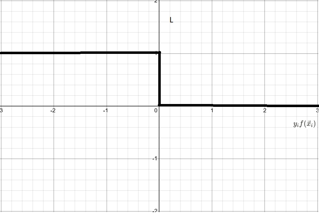
Hinge Loss formulation of SVM Suppose we consider the 0-1 loss for classification
L 01 ( y i , f ( x i ) ) = { 0 if y i f ( x ⃗ i ) > 0 1 if y i f ( x ⃗ i ) < 0 L_{01}(y_i,f(x_i)) = \begin{cases}
0 &\text{if } y_i f(\vec{x}_i) > 0 \\
1 &\text{if } y_i f(\vec{x}_i) < 0
\end{cases} L 01 ( y i , f ( x i )) = { 0 1 if y i f ( x i ) > 0 if y i f ( x i ) < 0 For the case of SVM, f ( x ⃗ i ) = y i ( w ⃗ ⊤ x ⃗ i + b ) f(\vec{x}_i) = y_i(\vec{w}^\top \vec{x}_i + b) f ( x i ) = y i ( w ⊤ x i + b )
So in order to do a correct classification, we want to
min 1 n ∑ i = 1 n L 01 ( y i , w ⃗ ⊤ x ⃗ i + b ) \min \frac{1}{n} \sum_{i=1}^n L_{01}(y_i, \vec{w}^\top \vec{x}_i + b) min n 1 i = 1 ∑ n L 01 ( y i , w ⊤ x i + b ) We cannot optimize this because it is not convex
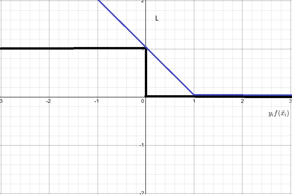
So we use hinge loss
L h i n g e ( y i , f ( x ⃗ i ) ) = max ( 1 − y i f ( x ⃗ i ) , 0 ) L_{hinge}(y_i, f(\vec{x}_i)) = \max(1-y_i f(\vec{x}_i),0) L hin g e ( y i , f ( x i )) = max ( 1 − y i f ( x i ) , 0 ) Hinge loss is the blue line here So now we have
min w ⃗ , b 1 n ∑ L h i n g e ( y i , w ⃗ ⊤ x ⃗ i + b ) + λ ∣ ∣ w ⃗ ∣ ∣ 2 2 \min_{\vec{w}, b} \frac{1}{n} \sum L_{hinge}(y_i, \vec{w}^\top \vec{x}_i + b) + \lambda ||\vec{w}||_2^2 w , b min n 1 ∑ L hin g e ( y i , w ⊤ x i + b ) + λ ∣∣ w ∣ ∣ 2 2 📌
We will see that this form of hinge loss formulation is exactly the same optimization problem as soft-margin SVM
Remember Soft-margin SVM formulation:
min w ⃗ , b , ξ ⃗ 1 2 ∣ ∣ w ⃗ ∣ ∣ 2 2 + C ( ∑ i = 1 n ξ i ) s.t. y i ( w ⃗ ⊤ x ⃗ i + b ) ≥ 1 − ξ i ξ i ≥ 0 \min_{\vec{w}, b, \vec{\xi}} \frac{1}{2}||\vec{w}||_2^2 + C(\sum_{i=1}^n \xi_i)\\
\text{s.t.} \\
y_i(\vec{w}^\top \vec{x}_i + b) \ge 1 - \xi_i \\
\xi_i \ge 0 w , b , ξ min 2 1 ∣∣ w ∣ ∣ 2 2 + C ( i = 1 ∑ n ξ i ) s.t. y i ( w ⊤ x i + b ) ≥ 1 − ξ i ξ i ≥ 0 Transform the formulation
min w ⃗ , b , ξ ⃗ 1 2 ∣ ∣ w ⃗ ∣ ∣ 2 2 + C ( ∑ i = 1 n ξ i ) s.t. ξ i ≥ max ( 1 − y i ( w ⃗ ⊤ x ⃗ i + b ) , 0 ) \min_{\vec{w}, b, \vec{\xi}} \frac{1}{2}||\vec{w}||_2^2 + C(\sum_{i=1}^n \xi_i)\\
\text{s.t.} \\
\xi_i \ge \max (1-y_i(\vec{w}^\top \vec{x}_i + b), 0) w , b , ξ min 2 1 ∣∣ w ∣ ∣ 2 2 + C ( i = 1 ∑ n ξ i ) s.t. ξ i ≥ max ( 1 − y i ( w ⊤ x i + b ) , 0 ) We can claim that at optimum, the constraint is tight (otherwise the objective function can be lowered)
min w ⃗ , b 1 2 ∣ ∣ w ⃗ ∣ ∣ 2 2 + C ( ∑ i = 1 n L 0 , 1 ( y i , w ⃗ ⊤ x ⃗ i + b ) ) \min_{\vec{w}, b} \frac{1}{2}||\vec{w}||_2^2 + C\bigg(\sum_{i=1}^n L_{0,1}(y_i, \vec{w}^\top \vec{x}_i + b)\bigg) w , b min 2 1 ∣∣ w ∣ ∣ 2 2 + C ( i = 1 ∑ n L 0 , 1 ( y i , w ⊤ x i + b ) ) Therefore if we let C = 1 2 n λ C = \frac{1}{2n \lambda} C = 2 nλ 1
Dual perspective of Soft-margin SVM L ( w ⃗ , b , ξ ⃗ , α ⃗ , β ⃗ ) = 1 2 ∣ ∣ w ⃗ ∣ ∣ 2 2 + C ∑ i = 1 n ξ i + ∑ i = 1 n α i ( ( 1 − ξ i ) − y i ( w ⃗ ⊤ x ⃗ i + b ) ) + ∑ i = 1 n β i ( − ξ i ) = 1 2 ∣ ∣ w ⃗ ∣ ∣ 2 2 − ∑ i = 1 n α i y i ( w ⃗ ⊤ x ⃗ i + b ) + ∑ i = 1 n α i + ∑ i = 1 n ( C − α i − β i ) ξ i \begin{split}
L(\vec{w},b,\vec{\xi},\vec{\alpha},\vec{\beta}) &= \frac{1}{2}||\vec{w}||_2^2 + C \sum_{i=1}^n \xi_i + \sum_{i=1}^n \alpha_i ((1-\xi_i) - y_i(\vec{w}^\top\vec{x}_i + b)) + \sum_{i=1}^n \beta_i (-\xi_i) \\
&=\frac{1}{2} ||\vec{w}||_2^2 - \sum_{i=1}^n \alpha_i y_i(\vec{w}^\top\vec{x}_i + b) + \sum_{i=1}^n \alpha_i + \sum_{i=1}^n (C-\alpha_i-\beta_i) \xi_i
\end{split} L ( w , b , ξ , α , β ) = 2 1 ∣∣ w ∣ ∣ 2 2 + C i = 1 ∑ n ξ i + i = 1 ∑ n α i (( 1 − ξ i ) − y i ( w ⊤ x i + b )) + i = 1 ∑ n β i ( − ξ i ) = 2 1 ∣∣ w ∣ ∣ 2 2 − i = 1 ∑ n α i y i ( w ⊤ x i + b ) + i = 1 ∑ n α i + i = 1 ∑ n ( C − α i − β i ) ξ i We have the primal and dual formulations:
p ∗ = min w ⃗ , b ⃗ , ξ ⃗ max α ⃗ , β ⃗ L ( ⋯ ) d ∗ = max α ⃗ , β ⃗ min w ⃗ , b ⃗ , ξ ⃗ L ( ⋯ ) p^* = \min_{\vec{w},\vec{b}, \vec{\xi}} \max_{\vec{\alpha}, \vec{\beta}} L(\cdots)
\\
d^* = \max_{\vec{\alpha}, \vec{\beta}} \min_{\vec{w},\vec{b}, \vec{\xi}} L(\cdots)
p ∗ = w , b , ξ min α , β max L ( ⋯ ) d ∗ = α , β max w , b , ξ min L ( ⋯ ) Consider first-order KKT conditions
∇ w ⃗ L = w ⃗ − ∑ α i y i x ⃗ i = 0 ⟹ w ⃗ = ∑ i = 1 n α i y i x ⃗ i \nabla_{\vec{w}} L = \vec{w} - \sum \alpha_i y_i \vec{x}_i = 0 \Longrightarrow \vec{w} = \sum_{i=1}^n \alpha_iy_i\vec{x}_i ∇ w L = w − ∑ α i y i x i = 0 ⟹ w = i = 1 ∑ n α i y i x i ∂ L ∂ b = − ∑ α i y i = 0 \frac{\partial L}{\partial b} = -\sum \alpha_i y_i = 0 ∂ b ∂ L = − ∑ α i y i = 0 ∂ L ∂ ξ i = C − α i − β i = 0 \frac{\partial L}{\partial \xi_i} = C - \alpha_i - \beta_i = 0 ∂ ξ i ∂ L = C − α i − β i = 0 Consider complementary slackness
α i ( ( 1 − ξ i ) − y i ( w ⃗ ⊤ x ⃗ i + b ) ) = 0 , ∀ i \alpha_i ((1-\xi_i) - y_i(\vec{w}^\top\vec{x}_i + b)) = 0, \forall i α i (( 1 − ξ i ) − y i ( w ⊤ x i + b )) = 0 , ∀ i β i ξ i = 0 \beta_i \xi_i = 0 β i ξ i = 0 Combining those equations,
if α i ≠ 0 \alpha_i \ne 0 α i = 0 α i ≠ C \alpha_i \ne C α i = C 0 < α i < C 0 < \alpha_i < C 0 < α i < C ( 1 − ξ i ) − y i ( w ⃗ ⊤ x ⃗ i + b ) = 0 (1-\xi_i) - y_i(\vec{w}^\top\vec{x}_i + b) = 0 ( 1 − ξ i ) − y i ( w ⊤ x i + b ) = 0 β i = C − α i \beta_i = C - \alpha_i β i = C − α i β i ≠ 0 \beta_i \ne 0 β i = 0 ξ i = 0 \xi_i = 0 ξ i = 0 y i ( w ⃗ ⊤ x ⃗ i + b ) = 1 y_i(\vec{w}^\top \vec{x}_i + b) = 1 y i ( w ⊤ x i + b ) = 1 Exactly on the margin! “Support vectors” if α i ≠ 0 , α i = C \alpha_i \ne 0, \alpha_i = C α i = 0 , α i = C C − α i − β i = − β i = 0 C-\alpha_i - \beta_i = -\beta_i = 0 C − α i − β i = − β i = 0 Then ξ i \xi_i ξ i Also, ( 1 − ξ i ) − y i ( w ⃗ ⊤ x ⃗ i + b ) = 0 (1-\xi_i) - y_i(\vec{w}^\top\vec{x}_i + b) = 0 ( 1 − ξ i ) − y i ( w ⊤ x i + b ) = 0 y i ( w ⃗ ⊤ x ⃗ i + b ) = 1 − ξ i ≤ 1 y_i(\vec{w}^\top\vec{x}_i + b) = 1-\xi_i \le 1 y i ( w ⊤ x i + b ) = 1 − ξ i ≤ 1 α i = 0 \alpha_i=0 α i = 0 β i = C ≠ 0 \beta_i = C \ne 0 β i = C = 0 ξ i = 0 \xi_i = 0 ξ i = 0 No margin violation Decision boundary not dependent on this point
The dual problem
L ( ⋯ ) = − 1 2 ( ∑ α i y i x ⃗ i ) ⊤ ( ∑ α i y i x ⃗ i ) + ∑ α i L(\cdots) = -\frac{1}{2} (\sum \alpha_i y_i\vec{x}_i)^\top(\sum \alpha_i y_i \vec{x}_i) + \sum \alpha_i L ( ⋯ ) = − 2 1 ( ∑ α i y i x i ) ⊤ ( ∑ α i y i x i ) + ∑ α i By substituting in KKT conditions
We have expressed the whole lagrangian in dual variables!
L ( ⋯ ) = − 1 2 [ α 1 y 1 ⋯ α n y n ] [ x ⃗ 1 ⊤ x ⃗ 2 ⊤ ⋮ x ⃗ n ⊤ ] [ x ⃗ 1 x ⃗ 2 ⋯ x ⃗ n ] [ α 1 y 1 ⋮ α n y n ] + ∑ α i = − 1 2 α ⃗ ⊤ d i a g ( y ⃗ ) X X ⊤ d i a g ( y ⃗ ) undefined Q α ⃗ + ∑ α i \begin{split}
L(\cdots) &= -\frac{1}{2}\begin{bmatrix}
\alpha_1 y_1 &\cdots &\alpha_ny_n
\end{bmatrix}
\begin{bmatrix}
\vec{x}_1^\top \\
\vec{x}_2^\top \\
\vdots \\
\vec{x}_n^\top
\end{bmatrix}
\begin{bmatrix}
\vec{x}_1 &
\vec{x}_2 &
\cdots &
\vec{x}_n
\end{bmatrix}
\begin{bmatrix}
\alpha_1 y_1 \\
\vdots \\
\alpha_n y_n
\end{bmatrix}
+ \sum \alpha_i \\
&=-\frac{1}{2} \vec{\alpha}^\top \underbrace{diag(\vec{y}) XX^\top diag(\vec{y})}_{Q} \vec{\alpha} + \sum \alpha_i
\end{split} L ( ⋯ ) = − 2 1 [ α 1 y 1 ⋯ α n y n ] ⎣ ⎡ x 1 ⊤ x 2 ⊤ ⋮ x n ⊤ ⎦ ⎤ [ x 1 x 2 ⋯ x n ] ⎣ ⎡ α 1 y 1 ⋮ α n y n ⎦ ⎤ + ∑ α i = − 2 1 α ⊤ Q d ia g ( y ) X X ⊤ d ia g ( y ) α + ∑ α i Kernels(Lifting) Instead of using
f ( x ⃗ ) = w ⃗ ⊤ x ⃗ + b f(\vec{x}) = \vec{w}^\top \vec{x}+b f ( x ) = w ⊤ x + b Use
f ( x ⃗ ) = w ⃗ ⊤ Φ ( x ⃗ ) + b f(\vec{x})=\vec{w}^\top\Phi(\vec{x})+b f ( x ) = w ⊤ Φ ( x ) + b
Interior Point Methods min f 0 ( x ⃗ ) s.t. f i ( x ⃗ ) ≤ 0 , ∀ i A x ⃗ = b ⃗ \min f_0(\vec{x}) \\
\text{s.t.} \\
f_i(\vec{x}) \le 0, \forall i \\
A\vec{x} = \vec{b} min f 0 ( x ) s.t. f i ( x ) ≤ 0 , ∀ i A x = b Conditions:
f i ( x ⃗ ) f_i(\vec{x}) f i ( x ) A ∈ R p × n A \in \mathbb{R}^{p \times n} A ∈ R p × n r a n k ( A ) = p rank(A) = p r ank ( A ) = p Problem is solvable, x ⃗ ∗ \vec{x}^* x ∗ Slater’s condition holds ⇒ strong duality
With those conditions, for optimal points, KKT conditions are neccesary and sufficient!
∃ x ⃗ ∗ , λ ⃗ ∗ , ν ⃗ ∗ s.t. A x ⃗ ∗ = b ⃗ , f i ( x ⃗ ∗ ) ≤ 0 , λ ⃗ ∗ ≥ 0 , ∇ f 0 ( x ⃗ ∗ ) + ∑ i = 1 m λ i ∗ ∇ f i ( x ⃗ ∗ ) + A ⊤ ν ⃗ ∗ = 0 , λ i ∗ ⋅ f i ( x ⃗ ∗ ) = 0 , ∀ i \exists \vec{x}^*, \vec{\lambda}^*, \vec{\nu}^* \text{ s.t.} \\
A\vec{x}^* = \vec{b}, f_i(\vec{x}^*) \le 0, \vec{\lambda}^* \ge 0, \\
\nabla f_0(\vec{x}^*) + \sum_{i=1}^m \lambda_i^* \nabla f_i(\vec{x}^*) + A^\top \vec{\nu}^* = 0, \\
\lambda_i^* \cdot f_i(\vec{x}^*) = 0, \forall i ∃ x ∗ , λ ∗ , ν ∗ s.t. A x ∗ = b , f i ( x ∗ ) ≤ 0 , λ ∗ ≥ 0 , ∇ f 0 ( x ∗ ) + i = 1 ∑ m λ i ∗ ∇ f i ( x ∗ ) + A ⊤ ν ∗ = 0 , λ i ∗ ⋅ f i ( x ∗ ) = 0 , ∀ i Those works for:
LPs, QPs, QCQP(Quadratic constrained quadratic programs), SOCPs, SDPs(Semi-definite programming)
Motivation:
Newton’s method ⇒ series of QPs Equality constrained ⇒ series of equality constrained QPs
🔥
Convert our problem to a series of equality constrained problems and remove inequality constraints ⇒ IPM
Barrier Function min A x ⃗ = b f 0 ( x ⃗ ) + ∑ i = 1 n I − ( f i ( x ⃗ ) ) \min_{A\vec{x} = b} f_0(\vec{x})+\sum_{i=1}^n I_-(f_i(\vec{x})) A x = b min f 0 ( x ) + i = 1 ∑ n I − ( f i ( x )) Where
I − : R → R s.t. I − = { 0 if u ≤ 0 ∞ if u > 0 I_-: \mathbb{R} \rightarrow \mathbb{R} \text{ s.t. } I_- = \begin{cases}
0 &\text{if } u\le 0\\
\infin &\text{if } u > 0
\end{cases} I − : R → R s.t. I − = { 0 ∞ if u ≤ 0 if u > 0 Can we make a differentiable convex approximation to this function?
I a p p r o x ( u ) = − 1 t log ( − u ) I_{approx}(u) = -\frac{1}{t} \log(-u) I a pp ro x ( u ) = − t 1 log ( − u ) Where t > 0 t > 0 t > 0 t t t
I a p p r o x I_{approx} I a pp ro x
Therefore we transformed the original problem into an approximate form, using logarithmic barrier function
ϕ ( x ⃗ ) = − ∑ i = 1 m log ( − f i ( x ⃗ ) ) \phi(\vec{x}) = -\sum_{i=1}^m \log(-f_i(\vec{x})) ϕ ( x ) = − i = 1 ∑ m log ( − f i ( x )) min A x ⃗ = b ⃗ f 0 ( x ⃗ ) + 1 t ϕ ( x ⃗ ) \min_{A\vec{x} = \vec{b}} f_0(\vec{x}) + \frac{1}{t} \phi(\vec{x}) A x = b min f 0 ( x ) + t 1 ϕ ( x ) Compute the gradient and hessian
∇ ϕ ( x ⃗ ) = ∑ i = 1 m − 1 f i ( x ⃗ ) ∇ f i ( x ⃗ ) \nabla \phi(\vec{x}) = \sum_{i=1}^m -\frac{1}{f_i(\vec{x})}\nabla f_i(\vec{x}) ∇ ϕ ( x ) = i = 1 ∑ m − f i ( x ) 1 ∇ f i ( x ) ∇ 2 ϕ ( x ⃗ ) = ∑ i = 1 m 1 f i ( x ⃗ ) 2 ∇ f i ( x ⃗ ) ∇ f i ( x ⃗ ) ⊤ + ∑ i = 1 m − 1 f i ( x ⃗ ) ∇ 2 f i ( x ⃗ ) \nabla^2 \phi(\vec{x}) = \sum_{i=1}^m \frac{1}{f_i(\vec{x})^2} \nabla f_i(\vec{x})\nabla f_i(\vec{x})^\top + \sum_{i=1}^m -\frac{1}{f_i(\vec{x})} \nabla^2 f_i(\vec{x}) ∇ 2 ϕ ( x ) = i = 1 ∑ m f i ( x ) 2 1 ∇ f i ( x ) ∇ f i ( x ) ⊤ + i = 1 ∑ m − f i ( x ) 1 ∇ 2 f i ( x ) Assume that this is solvable by Newton + unique solution
Solution: x ⃗ ∗ ( t ) \vec{x}^*(t) x ∗ ( t )
This solution should satisfy the KKT condition
A x ⃗ ∗ ( t ) = b , f i ( x ⃗ ∗ ( t ) ) < 0 , ∃ ν ⃗ ^ : t ⋅ ∇ f 0 ( x ⃗ ∗ ( t ) ) + ∇ ϕ ( x ⃗ ∗ ( t ) ) + A ⊤ ν ⃗ ^ = 0 A \vec{x}^*(t) = b, f_i(\vec{x}^*(t)) < 0, \\
\exists \hat{\vec{\nu}} : t \cdot \nabla f_0(\vec{x}^*(t)) + \nabla \phi(\vec{x}^*(t)) + A^\top \hat{\vec{\nu}} = 0 A x ∗ ( t ) = b , f i ( x ∗ ( t )) < 0 , ∃ ν ^ : t ⋅ ∇ f 0 ( x ∗ ( t )) + ∇ ϕ ( x ∗ ( t )) + A ⊤ ν ^ = 0 From this define
λ i ∗ ( t ) = − 1 t f i ( x ⃗ ∗ ( t ) ) , ν ⃗ ∗ ( t ) = ν ⃗ ^ / t \lambda_i^*(t) = -\frac{1}{t f_i(\vec{x}^*(t))}, \vec{\nu}^*(t) = \hat{\vec{\nu}}/t λ i ∗ ( t ) = − t f i ( x ∗ ( t )) 1 , ν ∗ ( t ) = ν ^ / t We claim that λ ⃗ ∗ , ν ⃗ ∗ \vec{\lambda}^*, \vec{\nu}^* λ ∗ , ν ∗
Let’s write the FOC condition of the transformed problem
t ⋅ ∇ f 0 ( x ⃗ ∗ ( t ) ) + ∑ − 1 f i ( x ⃗ ∗ ( t ) ) ⋅ ∇ f i ( x ⃗ ∗ ( t ) ) + A ⊤ ν ⃗ ^ = 0 ∇ f 0 ( x ⃗ ∗ ( t ) ) + ∑ λ i ∗ ( t ) ⋅ ∇ f i ( x ⃗ ∗ ( t ) ) + A ⊤ ν ∗ ( t ) = 0 t \cdot \nabla f_0(\vec{x}^*(t)) + \sum -\frac{1}{f_i(\vec{x}^*(t))} \cdot \nabla f_i(\vec{x}^*(t)) + A^\top \hat{\vec{\nu}} =0 \\
\nabla f_0(\vec{x}^*(t)) + \sum \lambda_i^*(t) \cdot \nabla f_i(\vec{x}^*(t)) + A^\top \nu^*(t) = 0 t ⋅ ∇ f 0 ( x ∗ ( t )) + ∑ − f i ( x ∗ ( t )) 1 ⋅ ∇ f i ( x ∗ ( t )) + A ⊤ ν ^ = 0 ∇ f 0 ( x ∗ ( t )) + ∑ λ i ∗ ( t ) ⋅ ∇ f i ( x ∗ ( t )) + A ⊤ ν ∗ ( t ) = 0 🔥
Notice that now this is the FOC of the lagrangian of the original problem!
Means ⇒ x ⃗ ∗ ( t ) \vec{x}^*(t) x ∗ ( t ) L ( x ⃗ , λ ⃗ ∗ ( t ) , ν ⃗ ∗ ( t ) ) L(\vec{x}, \vec{\lambda}^*(t), \vec{\nu}^*(t)) L ( x , λ ∗ ( t ) , ν ∗ ( t ))
not necessarily means that x ⃗ ∗ ( t ) \vec{x}^*(t) x ∗ ( t ) x ⃗ ∗ ( t ) \vec{x}^*(t) x ∗ ( t ) But we can derive a partial dual for the original problem
g ( λ ⃗ ∗ ( t ) , ν ⃗ ∗ ( t ) ) = min x ⃗ L ( x ⃗ , λ ⃗ ∗ ( t ) , ν ⃗ ∗ ( t ) ) = f 0 ( x ⃗ ∗ ( t ) ) + ∑ i = 1 m λ i ( t ) ⋅ f i ( x ⃗ ∗ ( t ) ) + ν ⃗ ∗ ( t ) ⊤ ( A x ⃗ ∗ ( t ) − b ⃗ ) = f 0 ( x ⃗ ∗ ( t ) ) − m t \begin{split}
g(\vec{\lambda}^*(t), \vec{\nu}^*(t)) &= \min_{\vec{x}} L(\vec{x}, \vec{\lambda}^*(t), \vec{\nu}^*(t)) \\
&= f_0(\vec{x}^*(t)) + \sum_{i=1}^m \lambda_i(t) \cdot f_i(\vec{x}^*(t))+\vec{\nu}^*(t)^\top (A\vec{x}^*(t)-\vec{b}) \\
&= f_0(\vec{x}^*(t)) -\frac{m}{t}
\end{split} g ( λ ∗ ( t ) , ν ∗ ( t )) = x min L ( x , λ ∗ ( t ) , ν ∗ ( t )) = f 0 ( x ∗ ( t )) + i = 1 ∑ m λ i ( t ) ⋅ f i ( x ∗ ( t )) + ν ∗ ( t ) ⊤ ( A x ∗ ( t ) − b ) = f 0 ( x ∗ ( t )) − t m Another way of stating λ i ( t ) = − 1 t f i ( x ⃗ ∗ ( t ) ) \lambda_i(t) = -\frac{1}{t f_i(\vec{x}^*(t))} λ i ( t ) = − t f i ( x ∗ ( t )) 1
− λ i ( t ) f i ( x ⃗ ∗ ( t ) ) = 1 t -\lambda_i(t) f_i(\vec{x}^*(t)) = \frac{1}{t} − λ i ( t ) f i ( x ∗ ( t )) = t 1 This is “approximate complementary slackness” ⇒ as t → ∞ t \rightarrow \infin t → ∞
Say I want accuracy ϵ \epsilon ϵ
Set ϵ = m t \epsilon = \frac{m}{t} ϵ = t m t = m ϵ t = \frac{m}{\epsilon} t = ϵ m
Barrier Methods Given strictly feasible x , t > 0 , μ > 1 , ϵ > 0 x, t > 0, \mu > 1, \epsilon >0 x , t > 0 , μ > 1 , ϵ > 0
Repeat:
CenteringCompute x ⃗ ∗ ( t ) \vec{x}^*(t) x ∗ ( t ) t f 0 ( x ⃗ ) + ϕ ( x ⃗ ) t f_0(\vec{x}) + \phi(\vec{x}) t f 0 ( x ) + ϕ ( x ) A x ⃗ = b ⃗ A\vec{x} = \vec{b} A x = b Starting at x ⃗ 1 \vec{x}_1 x 1 Update x ⃗ : = x ⃗ ∗ ( t ) \vec{x} := \vec{x}^*(t) x := x ∗ ( t ) Stopping critera: If m / t < ϵ m/t < \epsilon m / t < ϵ Increase t = μ ⋅ t t = \mu \cdot t t = μ ⋅ t