Some notes of GAN(Generative Adversarial Network) Specialization Course by Yunhao Cao(Github@ToiletCommander)

This work is licensed under a Creative Commons Attribution-NonCommercial-ShareAlike 4.0 International License.

Acknowledgements: Some of the resources(images, animations) are taken from:

1. Sharon Zhou & Andrew Ng and DeepLearning.AI’s GAN Specialization Course Track

2. articles on towardsdatascience.com

3. images from google image search(from other online sources)

Since this article is not for commercial use, please let me know if you would like your resource taken off from here by creating an issue on my github repository.

Last updated: 2022/6/14 15:07 CST

Generative Models

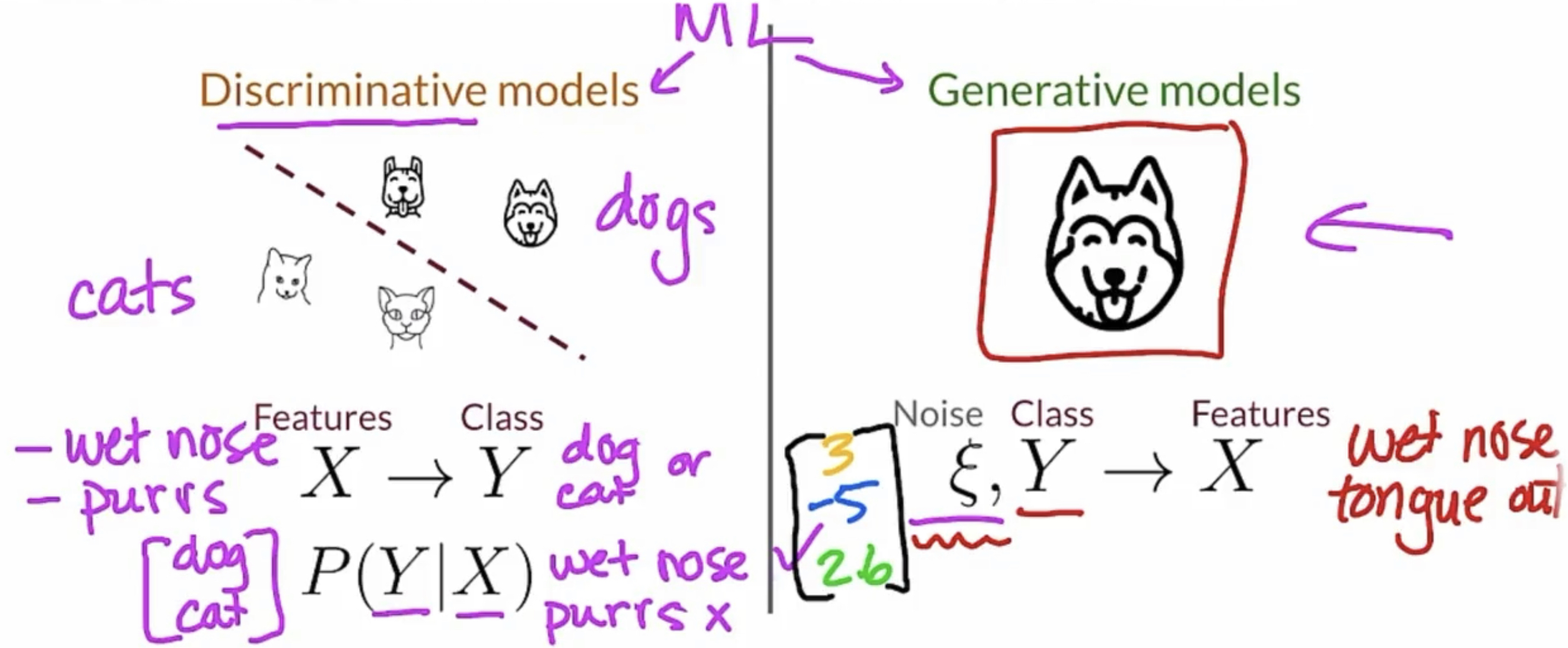
Different Generative Models

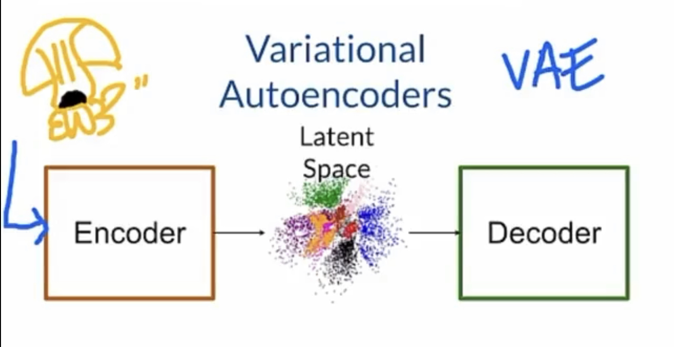
In a VAE model, two models, the encoder and the decoder is trained. The encoder tries to find a good representation of the image in the vector space (and hopefully same class rests in a cluster).

Variant: produce a linear subspace by the encoder, pick a random point from the subspace and feed it to decoder to kind of kick in the randomness of the image. The decoder’s job is to produce an image given a vector representation in the vector space.

During production, only the decoder is used. We take random point from the vector space and feed it to the decoder.

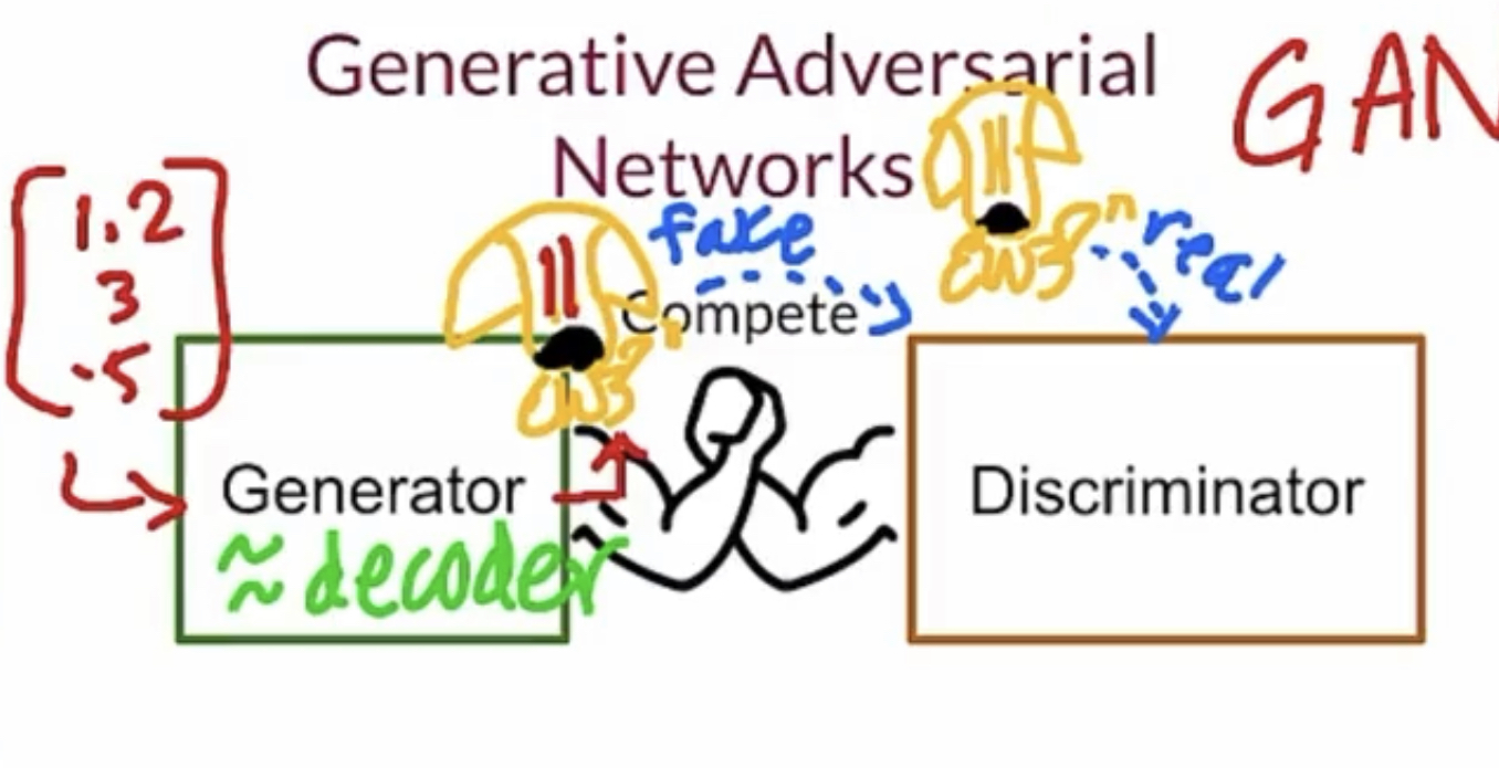
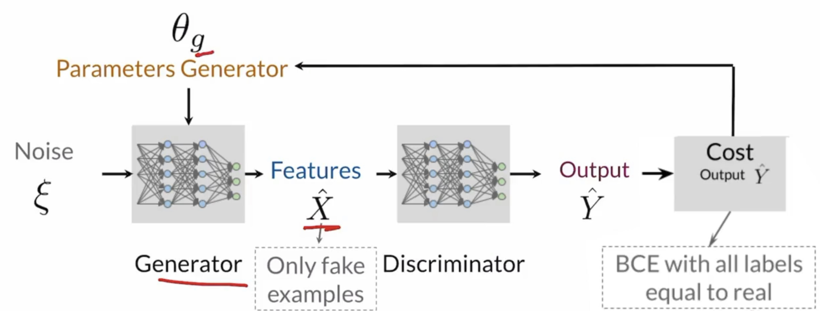
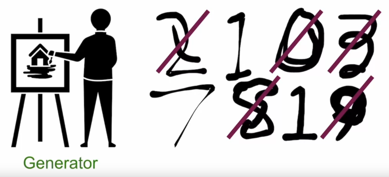
In a GAN model, two models, generator, and discriminator, are trained. Generator is used to generate fake images and try to fool the discriminator, while the goal of the discriminator is to train to recognize of two images which is the fake image generated by the generator.

Generator fights with discriminator and they competes with each other. Therefore the “adversarial” word is used to describe the model.

During production, the discriminator is removed and only the generator is used.

Therefore, the goal of GAN is to optimize the following problem:

Training A Basic GAN Network

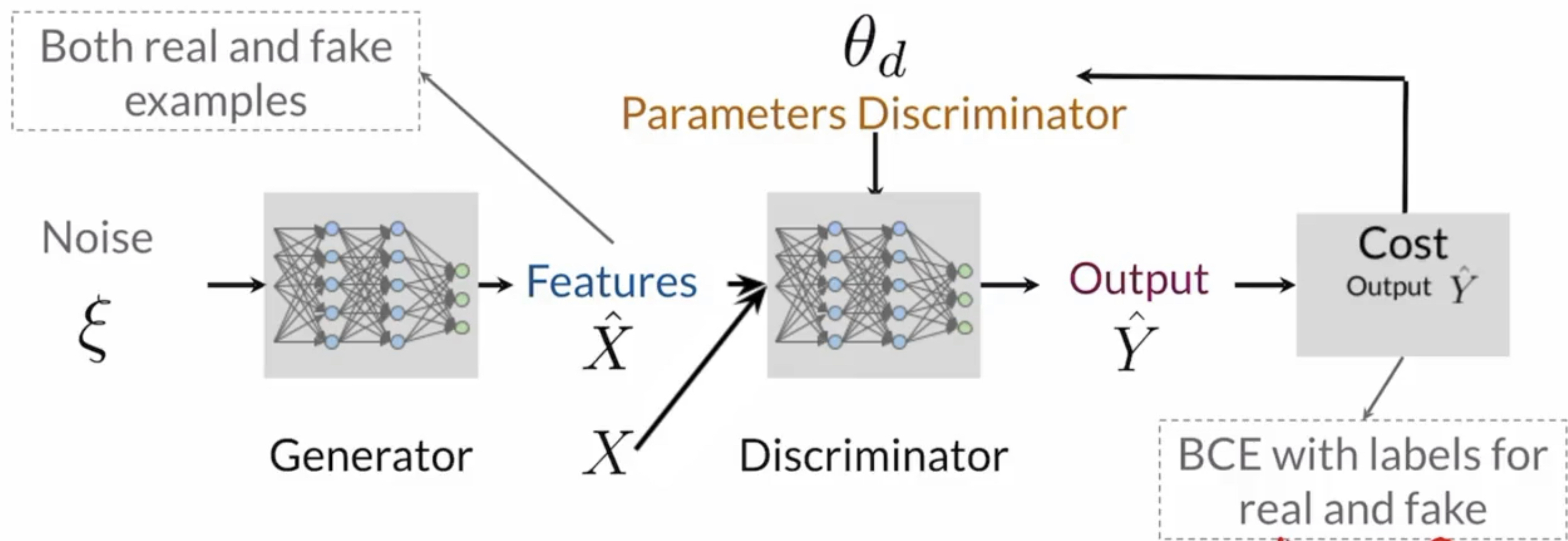
BCE Loss (Binary Classification Entropy Loss)

It is better than squared error because the loss is significantly higher when you misclassified the points, which helps to optimize the NN much faster.

Therefore, the goal is to optimize

DCGAN - Deep Convolution GAN

https://arxiv.org/pdf/1511.06434v1.pdf

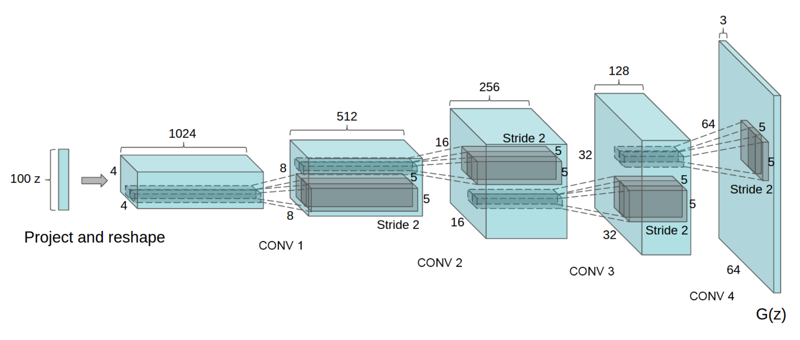
Generator

Basic Building Blocks

Generator Block:

ConvTranspose2D ⇒ BatchNorm ⇒ Relu

Last layer for Generator Block:

ConvTranspose2D ⇒ TanH

Architecture

Unsqeeze noise vector ⇒ 4 Generator Blocks, Upscaling Layers then Downscaling Layers, The Height and Width is always increasing since we’re doing transpose conv at every node.

Code

class Generator(nn.Module):
    '''
    Generator Class
    Values:
        z_dim: the dimension of the noise vector, a scalar
        im_chan: the number of channels in the images, fitted for the dataset used, a scalar
              (MNIST is black-and-white, so 1 channel is your default)
        hidden_dim: the inner dimension, a scalar
    '''
    def __init__(self, z_dim=10, im_chan=1, hidden_dim=64):
        super(Generator, self).__init__()
        self.z_dim = z_dim
        # Build the neural network
        self.gen = nn.Sequential(
            self.make_gen_block(z_dim, hidden_dim * 4),
            self.make_gen_block(hidden_dim * 4, hidden_dim * 2, kernel_size=4, stride=1),
            self.make_gen_block(hidden_dim * 2, hidden_dim),
            self.make_gen_block(hidden_dim, im_chan, kernel_size=4, final_layer=True),
        )

    def make_gen_block(self, input_channels, output_channels, kernel_size=3, stride=2, final_layer=False):
        '''
        Function to return a sequence of operations corresponding to a generator block of DCGAN, 
        corresponding to a transposed convolution, a batchnorm (except for in the last layer), and an activation.
        Parameters:
            input_channels: how many channels the input feature representation has
            output_channels: how many channels the output feature representation should have
            kernel_size: the size of each convolutional filter, equivalent to (kernel_size, kernel_size)
            stride: the stride of the convolution
            final_layer: a boolean, true if it is the final layer and false otherwise 
                      (affects activation and batchnorm)
        '''

        #     Steps:
        #       1) Do a transposed convolution using the given parameters.
        #       2) Do a batchnorm, except for the last layer.
        #       3) Follow each batchnorm with a ReLU activation.
        #       4) If its the final layer, use a Tanh activation after the deconvolution.

        # Build the neural block
        if not final_layer:
            return nn.Sequential(
                #### START CODE HERE ####
                nn.ConvTranspose2d(input_channels,output_channels,kernel_size,stride),
                nn.BatchNorm2d(output_channels),
                nn.ReLU()
                #### END CODE HERE ####
            )
        else: # Final Layer
            return nn.Sequential(
                #### START CODE HERE ####
                nn.ConvTranspose2d(input_channels,output_channels,kernel_size,stride),
                nn.Tanh()
                #### END CODE HERE ####
            )

    def unsqueeze_noise(self, noise):
        '''
        Function for completing a forward pass of the generator: Given a noise tensor, 
        returns a copy of that noise with width and height = 1 and channels = z_dim.
        Parameters:
            noise: a noise tensor with dimensions (n_samples, z_dim)
        '''
        return noise.view(len(noise), self.z_dim, 1, 1)

    def forward(self, noise):
        '''
        Function for completing a forward pass of the generator: Given a noise tensor, 
        returns generated images.
        Parameters:
            noise: a noise tensor with dimensions (n_samples, z_dim)
        '''
        x = self.unsqueeze_noise(noise)
        return self.gen(x)

def get_noise(n_samples, z_dim, device='cpu'):
    '''
    Function for creating noise vectors: Given the dimensions (n_samples, z_dim)
    creates a tensor of that shape filled with random numbers from the normal distribution.
    Parameters:
        n_samples: the number of samples to generate, a scalar
        z_dim: the dimension of the noise vector, a scalar
        device: the device type
    '''
    return torch.randn(n_samples, z_dim, device=device)

Discriminator

Basic Building Block

Discriminator Block:

Conv2D ⇒ BatchNorm ⇒ LeakyReLU(0.2)

Last Layer of Discriminator Block:

Conv2D ⇒ 1x1x1 ⇒ Sigmoid

Architecture

Input Image ⇒ Discriminator Block * 3 (Upscaling # layers in the first and second block, downscaling to 1 layer in the third block)

Code

# UNQ_C3 (UNIQUE CELL IDENTIFIER, DO NOT EDIT)
# GRADED FUNCTION: Discriminator
class Discriminator(nn.Module):
    '''
    Discriminator Class
    Values:
        im_chan: the number of channels in the images, fitted for the dataset used, a scalar
              (MNIST is black-and-white, so 1 channel is your default)
    hidden_dim: the inner dimension, a scalar
    '''
    def __init__(self, im_chan=1, hidden_dim=16):
        super(Discriminator, self).__init__()
        self.disc = nn.Sequential(
            self.make_disc_block(im_chan, hidden_dim),
            self.make_disc_block(hidden_dim, hidden_dim * 2),
            self.make_disc_block(hidden_dim * 2, 1, final_layer=True),
        )

    def make_disc_block(self, input_channels, output_channels, kernel_size=4, stride=2, final_layer=False):
        '''
        Function to return a sequence of operations corresponding to a discriminator block of DCGAN, 
        corresponding to a convolution, a batchnorm (except for in the last layer), and an activation.
        Parameters:
            input_channels: how many channels the input feature representation has
            output_channels: how many channels the output feature representation should have
            kernel_size: the size of each convolutional filter, equivalent to (kernel_size, kernel_size)
            stride: the stride of the convolution
            final_layer: a boolean, true if it is the final layer and false otherwise 
                      (affects activation and batchnorm)
        '''
        #     Steps:
        #       1) Add a convolutional layer using the given parameters.
        #       2) Do a batchnorm, except for the last layer.
        #       3) Follow each batchnorm with a LeakyReLU activation with slope 0.2.
        #       Note: Don't use an activation on the final layer
        
        # Build the neural block
        if not final_layer:
            return nn.Sequential(
                #### START CODE HERE ####
                nn.Conv2d(input_channels,output_channels,kernel_size,stride),
                nn.BatchNorm2d(output_channels),
                nn.LeakyReLU(0.2)
                #### END CODE HERE ####
            )
        else: # Final Layer
            return nn.Sequential(
                #### START CODE HERE ####
                nn.Conv2d(input_channels,output_channels,kernel_size,stride)
                #### END CODE HERE ####
            )

    def forward(self, image):
        '''
        Function for completing a forward pass of the discriminator: Given an image tensor, 
        returns a 1-dimension tensor representing fake/real.
        Parameters:
            image: a flattened image tensor with dimension (im_dim)
        '''
        disc_pred = self.disc(image)
        return disc_pred.view(len(disc_pred), -1)

Mode Collapse

Mode Definition

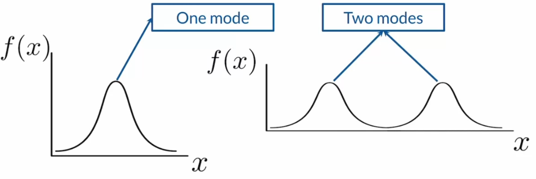
Mode is the area where PDF is max, it marks the value on which $P(X \in dx)$ is max (the most frequent number).

Mode Collapse Problem

Think about in high dimensional space, each class has a normal distribution with some values concentrated at its modes, like below.

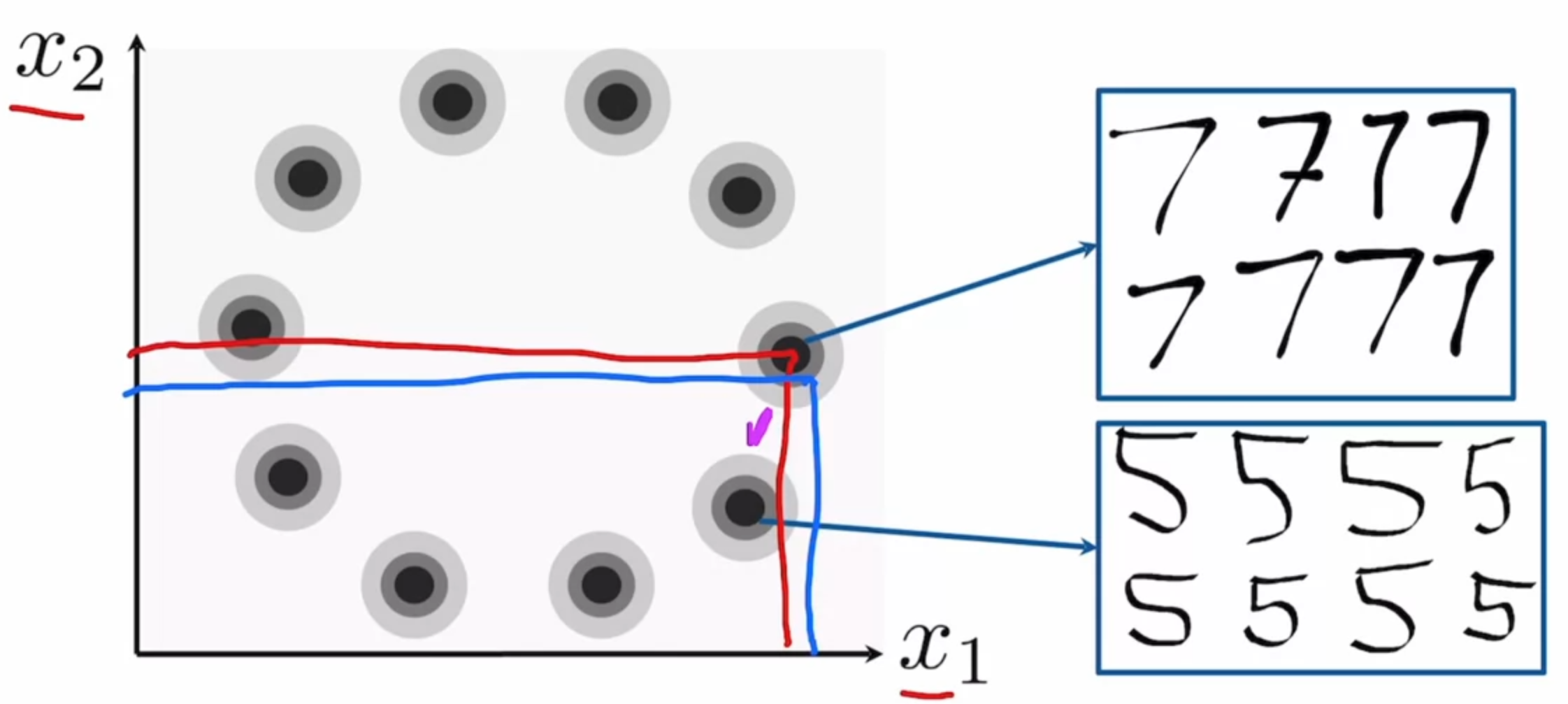
Think about a discriminator that has been trained pretty well but just does not determine well enough on some of the classes (in this case, 1 and 7).

This means the discriminator is probably stuck in a local minima.

Now the generator knows that generating the classes of images that the discriminator is weak at will help fool the discriminator.

So therefore the Generator outputs those classes of images

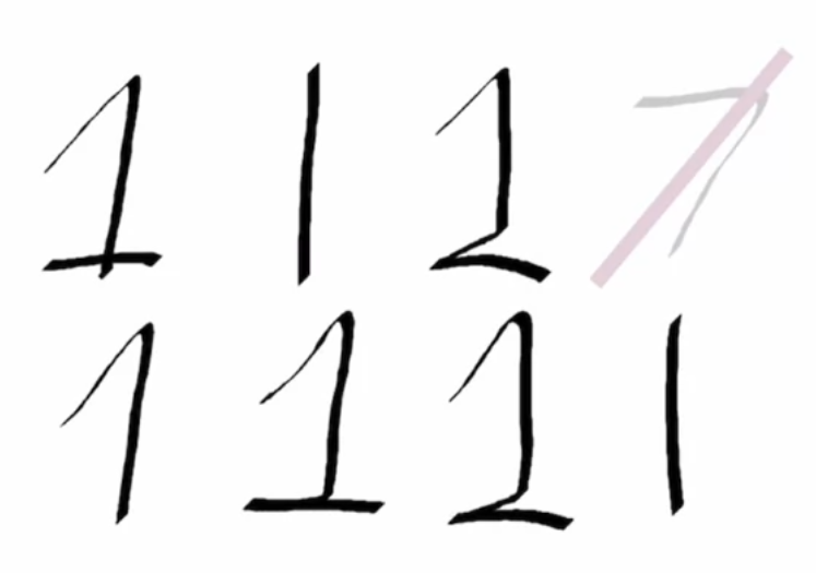
Since the discriminator is stuck in a local optima, it keeps telling generator that the generated images are “real”, though there might be little difference in its ability to determine one class from other among those weak classes (in this case 7 > 1).

Therefore the generator learns to produce classes of images of only 1s ⇒ The Generator is stuck in one mode, therefore it is called mode collapse.

Vanishing Gradient Problem for BCE Loss

https://arxiv.org/pdf/1701.04862.pdf

Reminder:

Goal of generator:

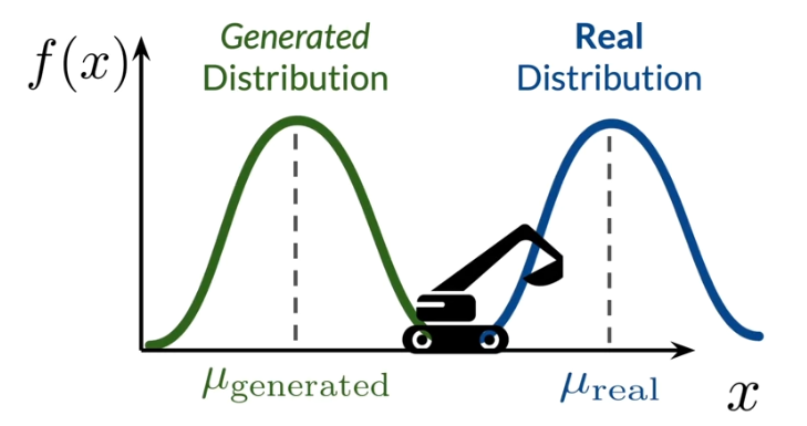
Approximate real distribution

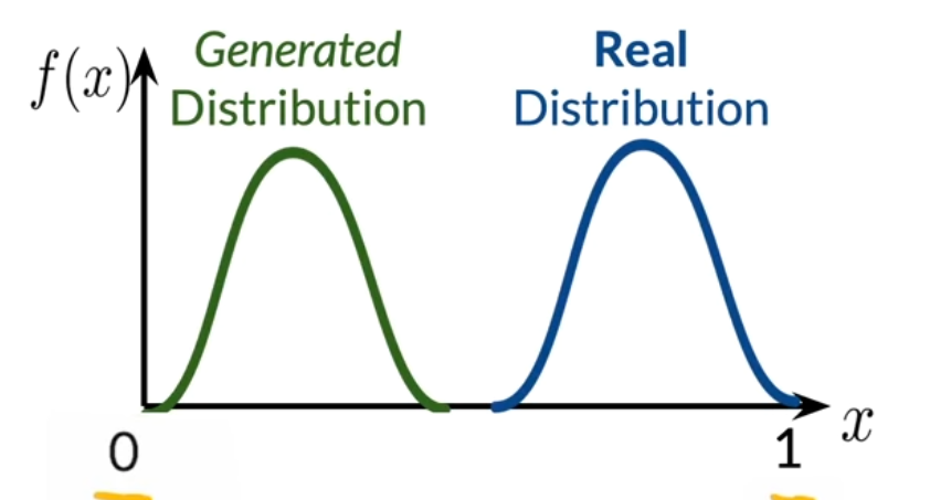
However, Goal of Discriminator:

Given x, tell apart whether x belongs to the generated distribution or the real distribution.

Well, looks like they are pretty clear & straight forward optimization problems, what is the problem here?

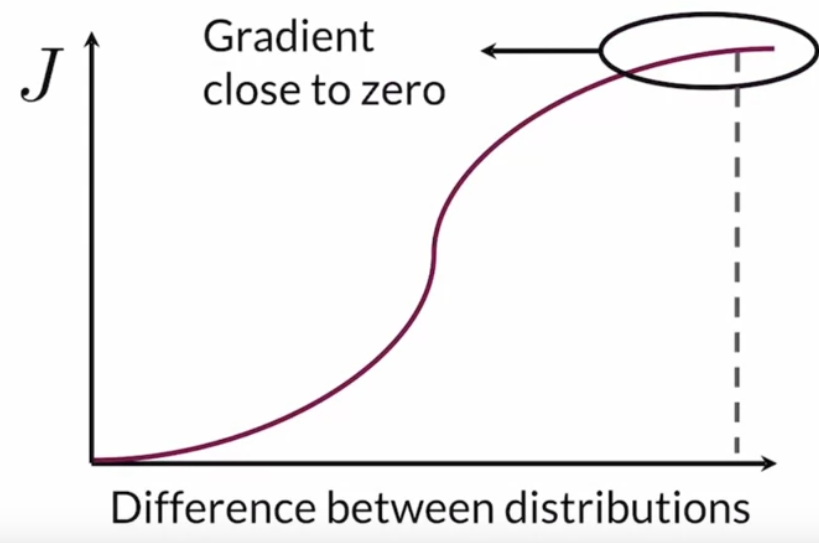
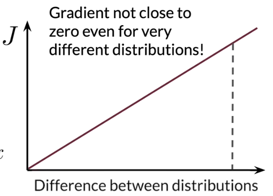
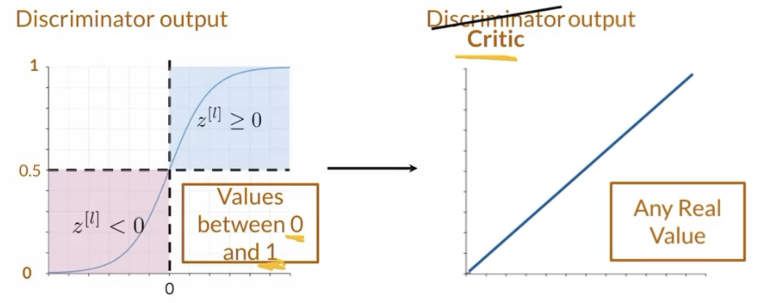
As discriminator is more and more powerful, the descriminator with BCE Loss provides less and less gradient to the generator to optimize. And we have the problem of vanishing gradient in the end.

Where $a \odot b$ denotes the element-wise product of a and b

Earth Mover’s Distance

Earth Mover’s Distance describes the Effort needed to make the generated distribution to the real distribution.

Wassertain Loss

Approximates Earth Mover’s Distance

Before we introduce the W-Loss, we will see GAN as a min-max game

Where $g(\cdot)$ is the generator function, and $d(\cdot)$ is the discriminator function.

Instead of the logarithm in the cost function $J$, the W-Loss is formulated as:

Conditioning on W-Loss

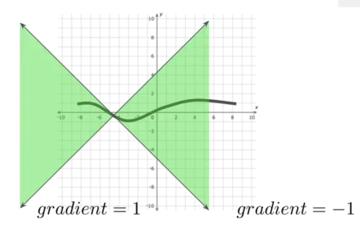
1. has to be 1-Lipschitz continuous.
   1. Norm of the gradient has to always be $\le 1$: $\forall x, ||\nabla f(x)||_2 \le 1$

1-L Continuous Enforcement

Weight Clipping

1. However, may limit the ability to learn.

2. Regularization
   1. Change the min-max to
   2. $\min_{g} \max_{d} \mathbb{E}[d(x)]-\mathbb{E}[d(g(x))] + \lambda reg$, where $reg$ is the regularization term
   3. tends to work better

Regularization Term is done by…

first interpolating a $\hat{x}$ by applying a $\epsilon$ and $1 - \epsilon$ to real and fake images

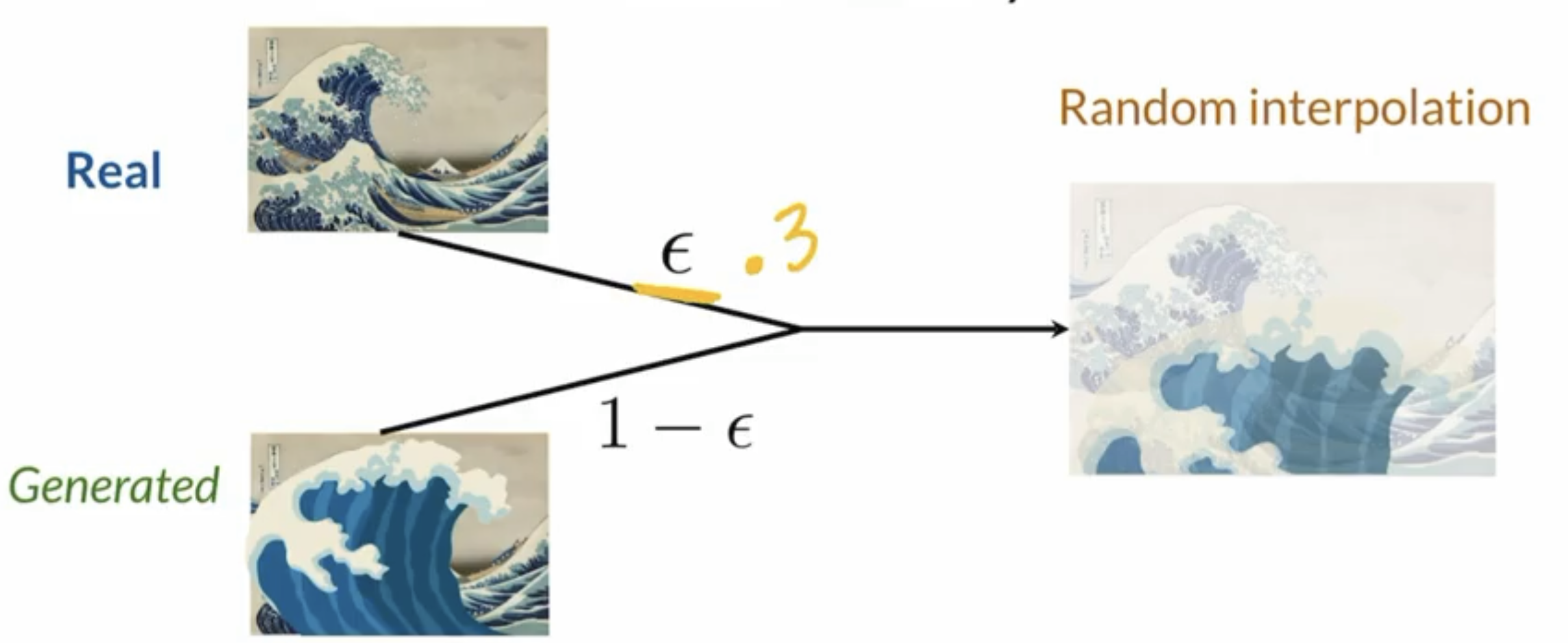
Then

Conditional GAN

All Above models are unconditional GANs

Now we want to be able to secify which type of product to generate, so we train the GAN with labeled dataset.

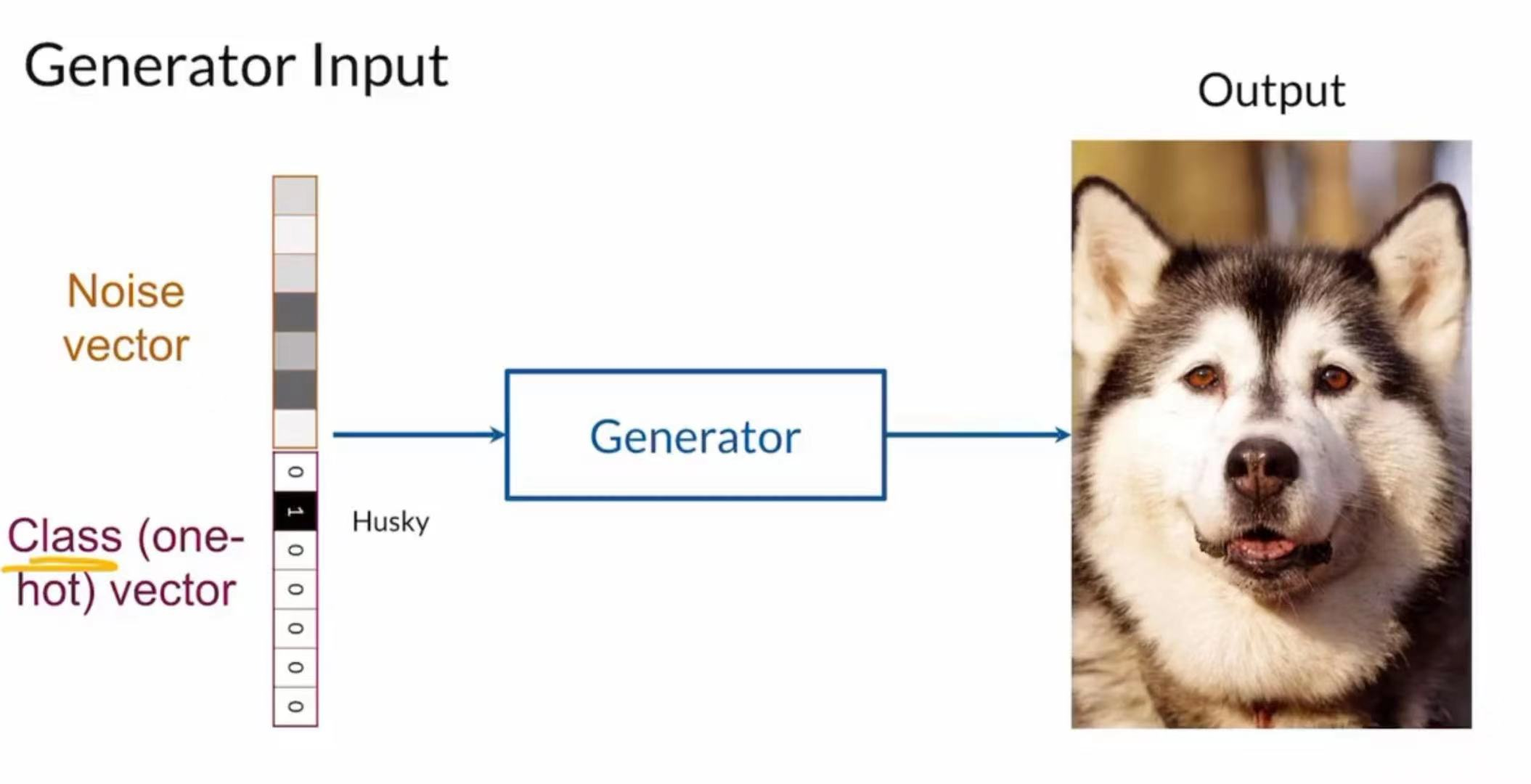
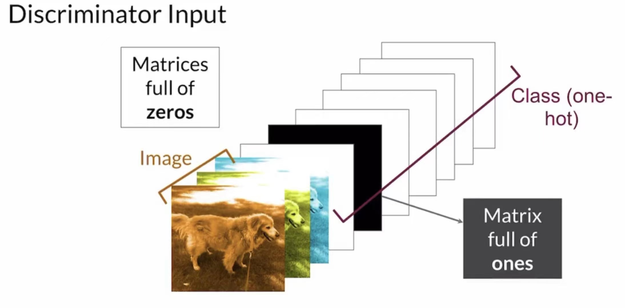
In the previous networks we had a noise vector as the input to the generator, we will now add an one-hot vector to the generator. For the discriminator give images as well as a label (one-hot as additional channels) and the discriminator will still output a probability.

There are ways to compress data in the discriminator input. But this uncompressed way definitely work.

Controllable Generation

It’s different from conditional generation

1. Now we control the feature, not the class

2. We don’t have to modify the network structures

3. Training dataset doesn’t need to be labeled

4. Tweaking the noise vector $\vec{z}$ to change feature, while conditional generation alters the model input.

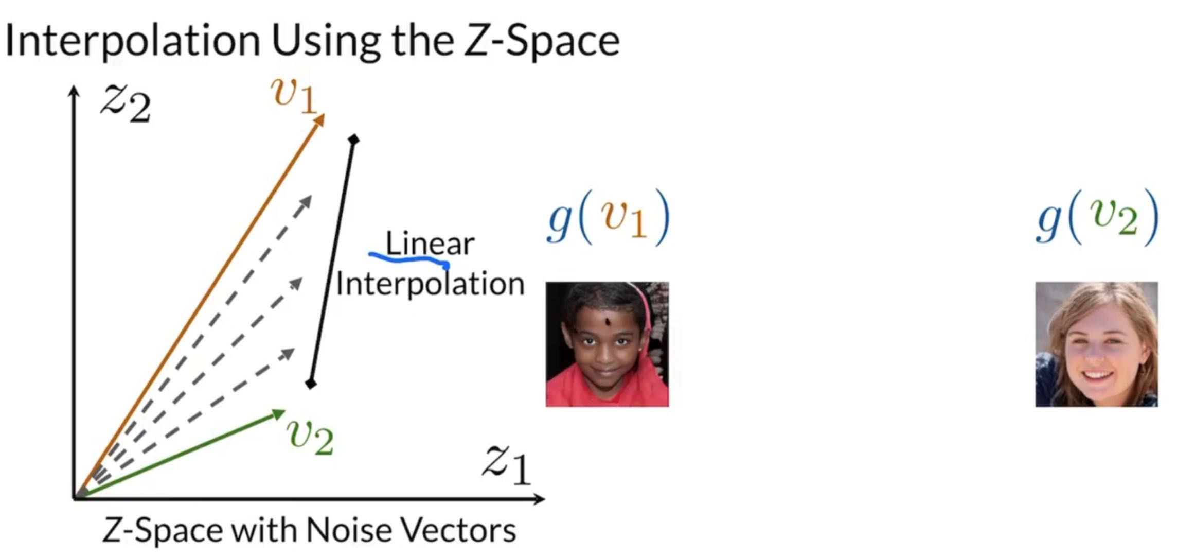
After training, observe the output of two z space vectors $v_1$ and $v_2$, and we can interpolate the vectors and get an intermediate result (we can do linear interpolation but there are also other interpolation methods)

Problems

Feature Correlation

Sometimes we will want to alter a feature that has high correlation with other features, for example adding a beard. But beard might be tied to masculinity so it might be possible to not be able to just change the beard without changing the degree of masculinity.

Z-Space Entanglement

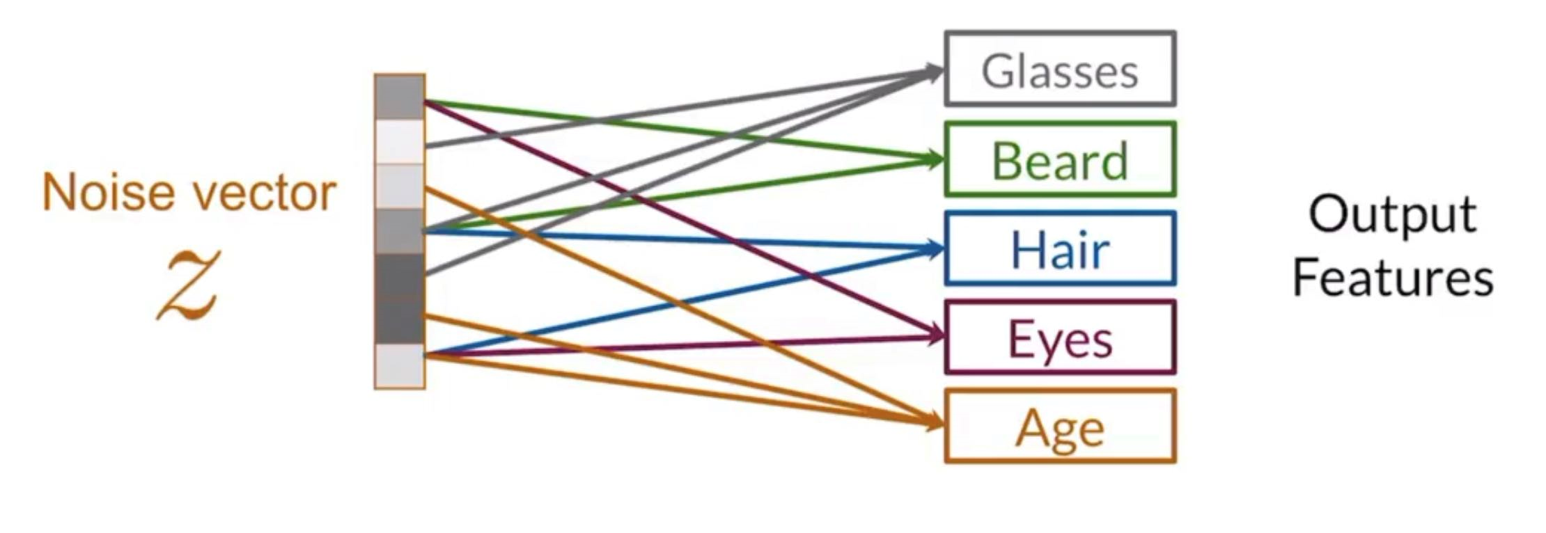
Sometimes modifying a direction in noise vector we might change multiple features at the same time. This usually happens when z-space don’t have enough dimensions to map one feature at a time.

Classifier Gradients as a method of finding z-space direciton to change a feature

We use a trained classifier to classify a generated image, $g(\vec{z})$ produced by the generator, and we use the classifier to classify if the image contains the feature of not, given by $d(g(\vec{z}))$. We can repeat this process until the feature is present in the image by continuously modifying the noise vector $\vec{z}$ in the direction of the gradient, $\nabla_{\vec{z}} d(g(\vec{z}))$. Finally once the classifier says YES, we will use a weighted average of the direction we have stepped through to change the feature later.

Disentanglement Methods

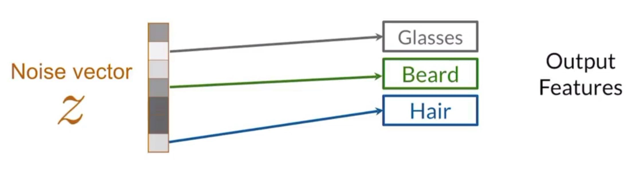
Supervision

1. Just like what we did for the conditional GAN, we would add labeled data but this time instead of adding one-hot to the generator the information would be embbeded into the noise vector itself.

Loss Function

Add a regularization term (BCE or W-Loss) to encourage each index of the noise vector to be associated with some feature.

There are techniques to do this in an unsupervised way.