Some notes of GAN(Generative Adversarial Network) Specialization Course by Yunhao Cao(Github@ToiletCommander)

This work is licensed under a Creative Commons Attribution-NonCommercial-ShareAlike 4.0 International License.

Acknowledgements: Some of the resources(images, animations) are taken from:

1. Sharon Zhou & Andrew Ng and DeepLearning.AI’s GAN Specialization Course Track

2. articles on towardsdatascience.com

3. images from google image search(from other online sources)

Since this article is not for commercial use, please let me know if you would like your resource taken off from here by creating an issue on my github repository.

Last updated: 2022/6/16 14:15 CST

Evaluating a GAN

Evaluating is a challenging task because..

1. GANs are learning to composing not singing - it is hard to determine if it was right or wrong
   1. Classifiers have labeled data to compare against

2. Although in a GAN there are real or fake images, the discriminators in GAN always overfits to the generators and there’s not a universal discriminator that compares two different generators

But we can compare images

We compare several images generated by GANs in terms of their fidelity and diversity. But it can be challenging.

Pixel Distance

Works, but not reliable

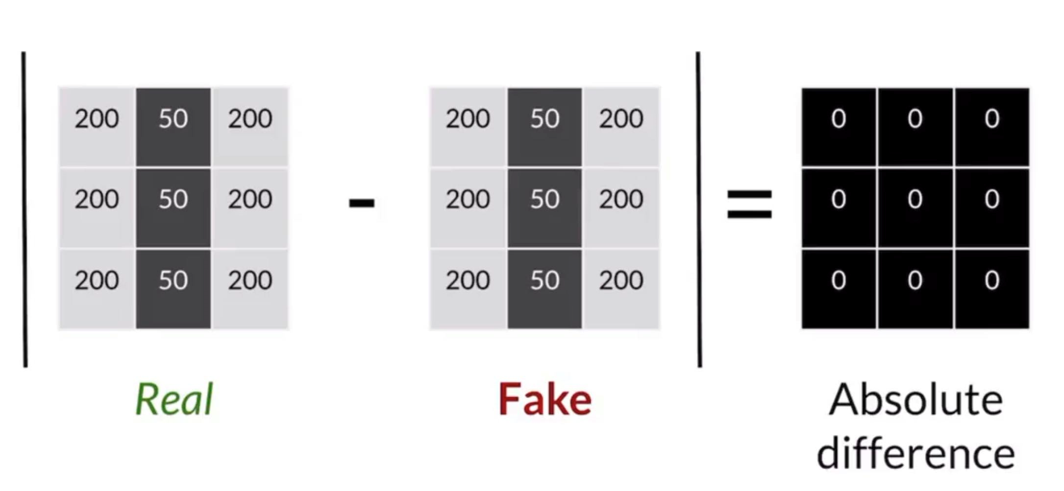
Imagine the fake image shifted one pixel to the right, then the whole pixel distance is huge and exaggerated though the two images are similar.

Feature Distance

Less Sensitive to small shifts,

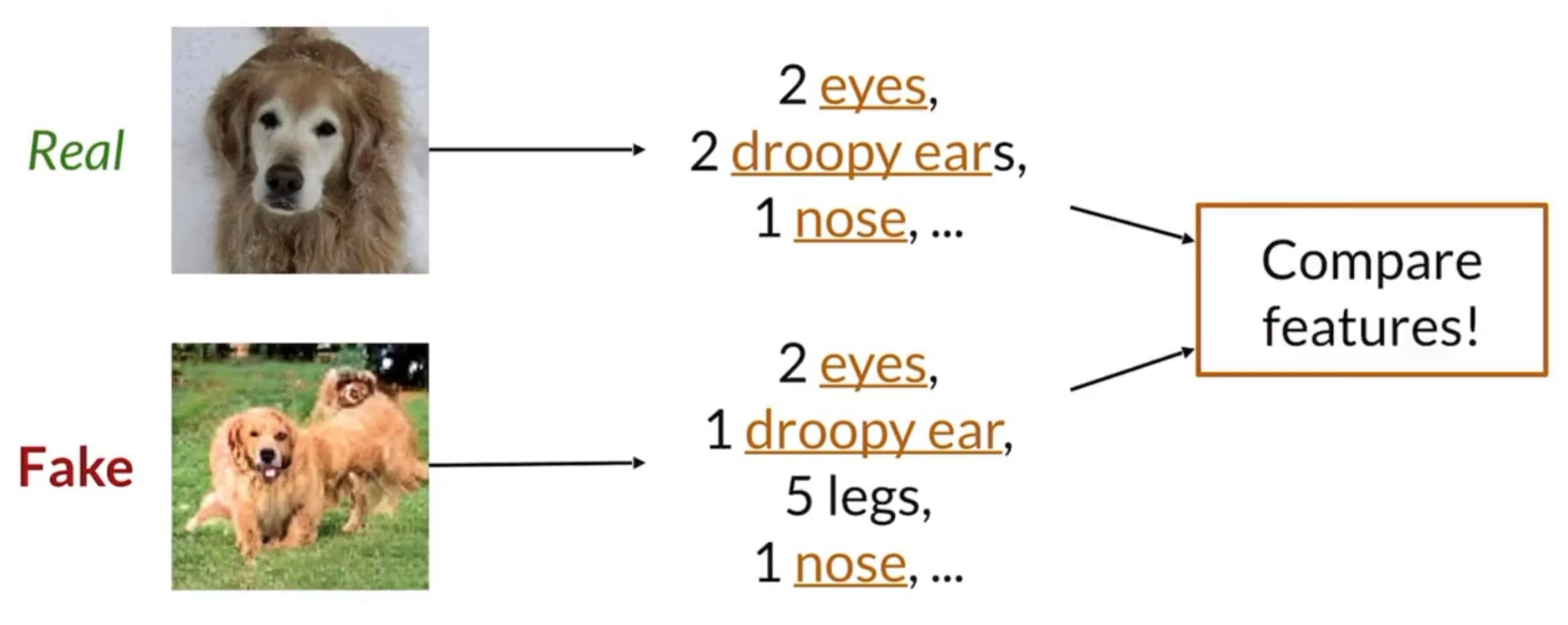
Extract information about the real and fake images and then compare the features (high-level semantic information)

Usually the classifier we use is Inception network (Sharon mentioned Inception-V3, which has 42 layers deep but very computationally efficient, but I think the newest is now Inception v4)

Frechet Distance and Frechet Inception Distance

the Frechet Distance is developed to compare distance between curves but can be modified to measure distance between distributions as well.

We will use the classic dogwalker schenerio to illustrate this concept

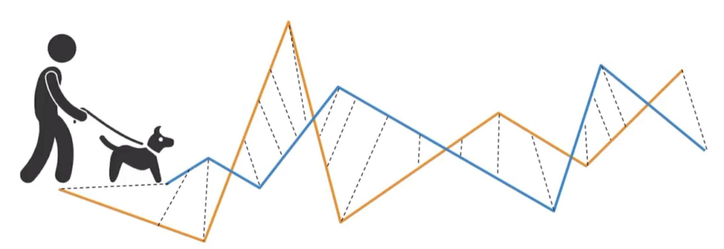
1. Both the dogwalker and the dog is walking

2. they can run in different speeds

3. they can run in different directions

4. but neither of them can run backwards

figure out the minimum leash length needed to walk from beginning to end ⇒ what is the minimum leash needed to walk the curves without giving him more slack during the walk.

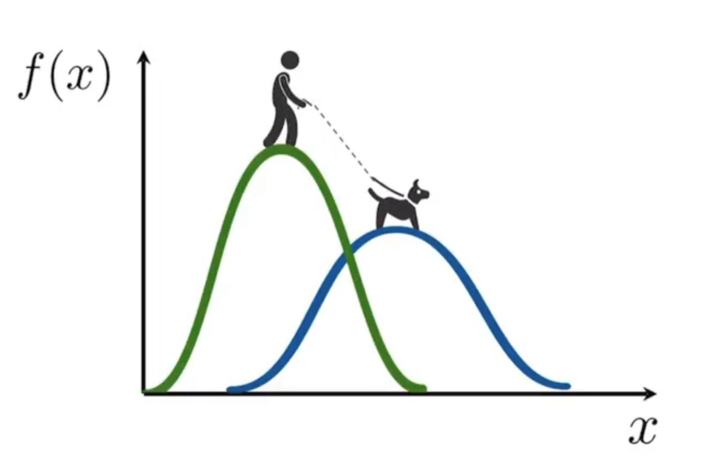
We can also determine the Frechet Distance between univariate normal distributions using a similar idea.

On a multivariate Normal distribution, the Frechet Distance looks like:

Where $Tr(\cdot)$ is the trace of a matrix (sum of diagonal terms)

And the square root is square root on matrix, not on each element

The above formula is also called Frechet Inception Distance (FID), one of the most commonly used matrix to evaluate embeddings of real and fake images. The lower FID is, it means the closer fake image distributions are to the real image distributions.

Shortcomings of FID

1. Uses pre-trained Inception model which may not capture all features

2. Needs a large sample size

3. Slow to run

4. Limited statistics used: only mean and sd.

Inception Score

1. Now replaced by FID

2. But reported in many papers so good to know

3. Keeps calssifier intact and don’t use any intermediate values
   1. Directly see the output of Inception network
   2. If a score for an exact class is high $P(y|X)$, it means the image is arguably high fidelity since it is easier to recognize and resembles features that is closer to one class.
   3. Look across many samples and see that the generator is generating many different classes or not $P(y)$

So, single score KL Divergence

Tries to measure how much information you can gain on $P(y|X)$ given just information about $P(y)$.

So...inception score

But

1. Can be exploited or gamed
   1. Generate one realistic image of each class

2. Only looks at fake images
   1. No comparison to real images

3. Can miss useful features
   1. ImageNet isn’t everything

Ways to sample images for comparison

1. For real, we usually just sample uniformly from the data

2. For fake, since we would use a normal distribution to generate noise vector $\vec{z}$s, we can also use the same distribution to generate fakes for comparison, but with some tricks.
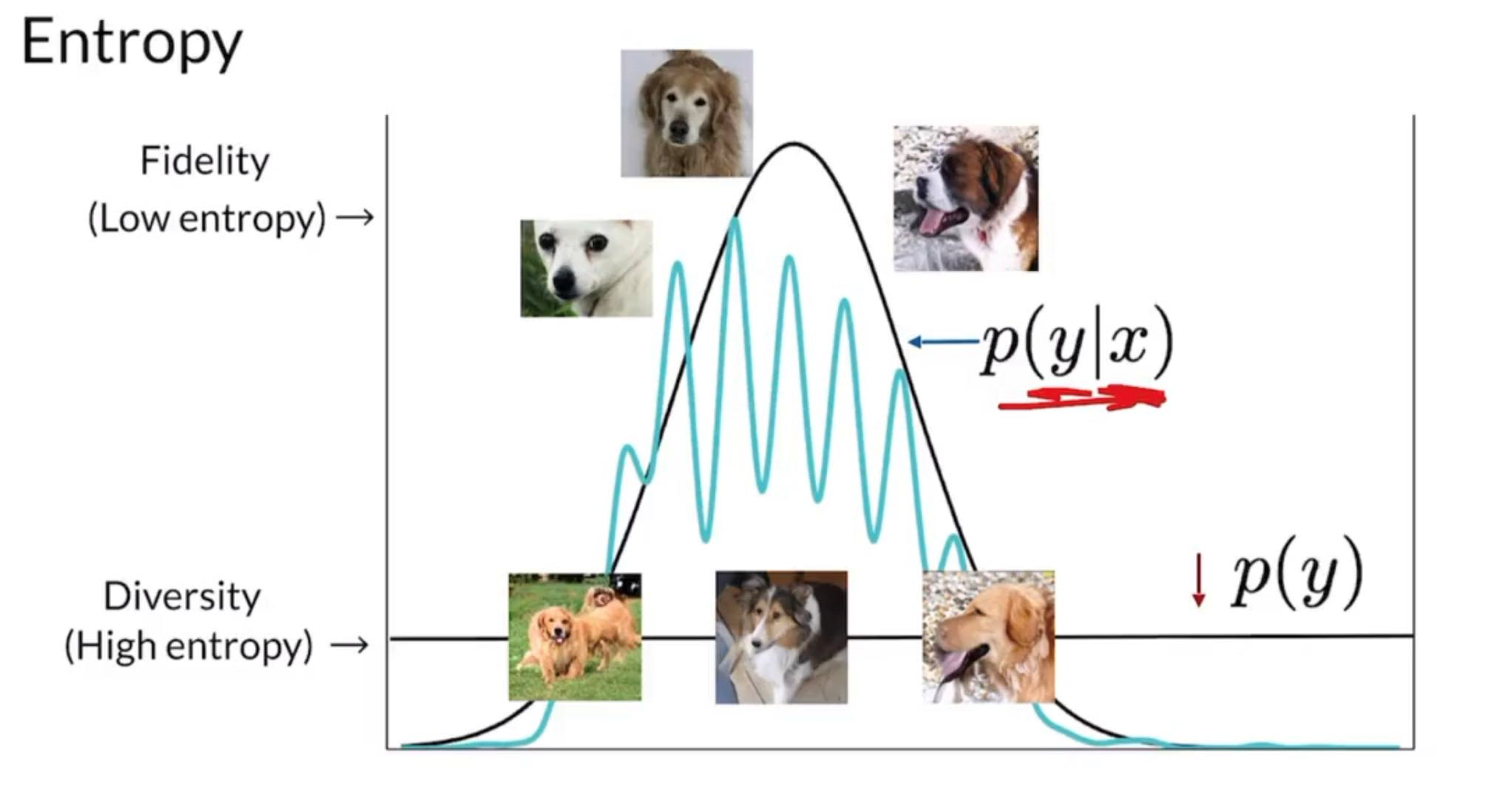
   1. There’s a tradeoff between fidelity and diversity
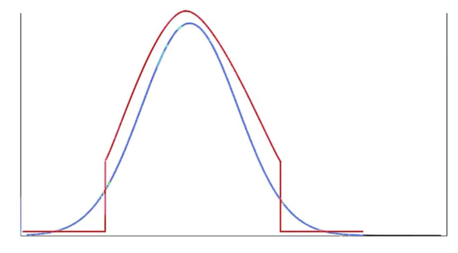
   2. If we sample closer to the middle, we will improve the fidelity of sampled fakes since those are the values that occured more in training, but we lost diversity since we gave up certain regions of $\vec{z}$s.
   3. Truncation Trick

   

Precision and Recall

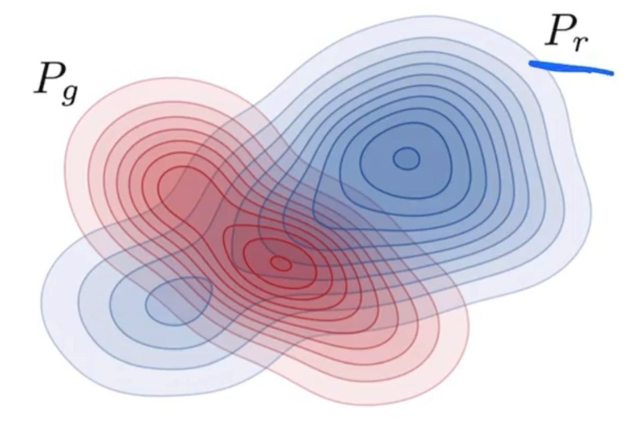
In a GAN network, we want the generated image distribution (fake distribution) $P_g$ to match exactly with the distribution of $P_r$ (not a subset, not a super-set, but exactly equal)

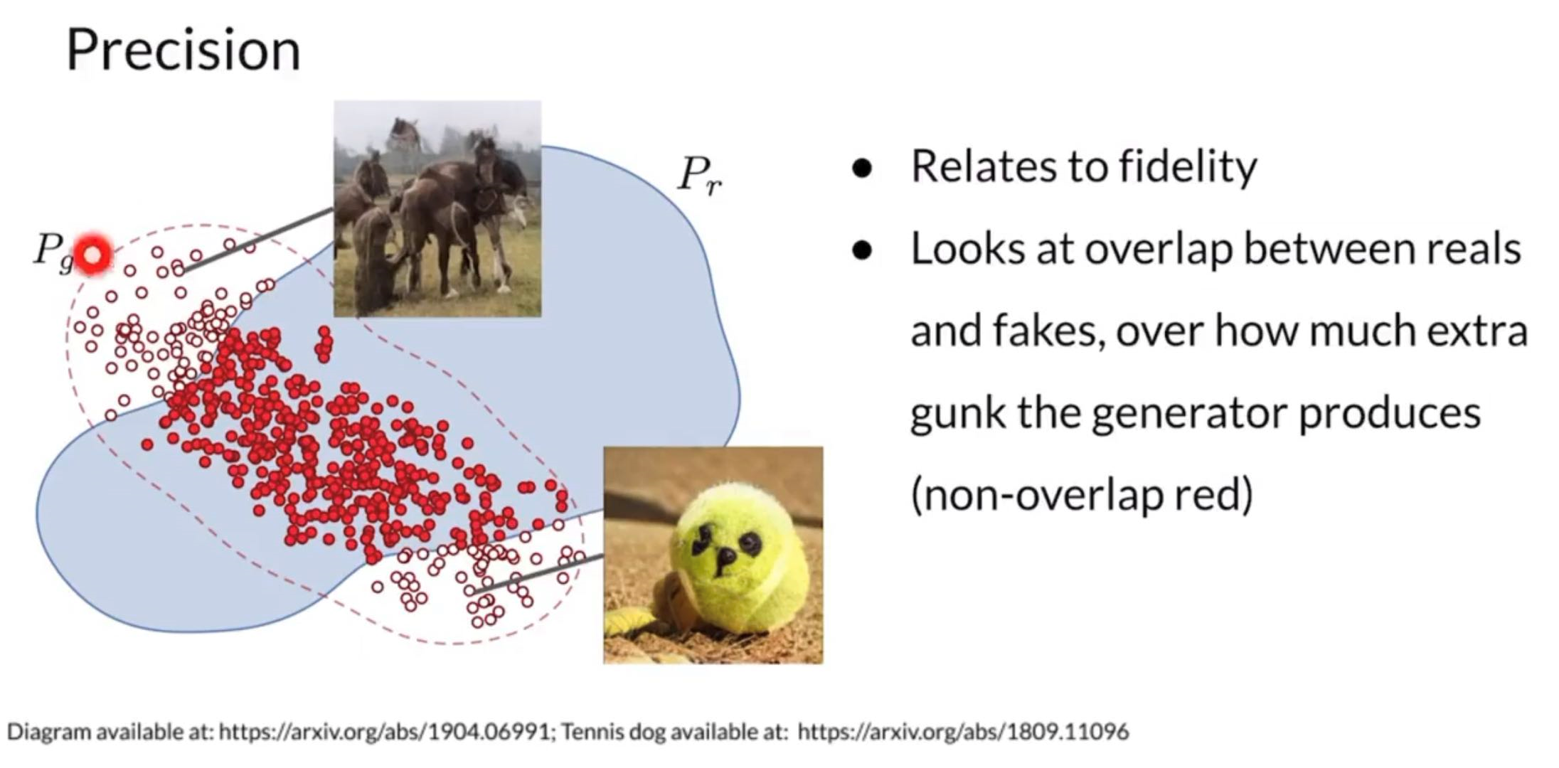
Percision: area of fake distribution overlapping with the real distribution divided by area of fake distribution. Percentage of fakes that look real ⇒ quality of generated fakes

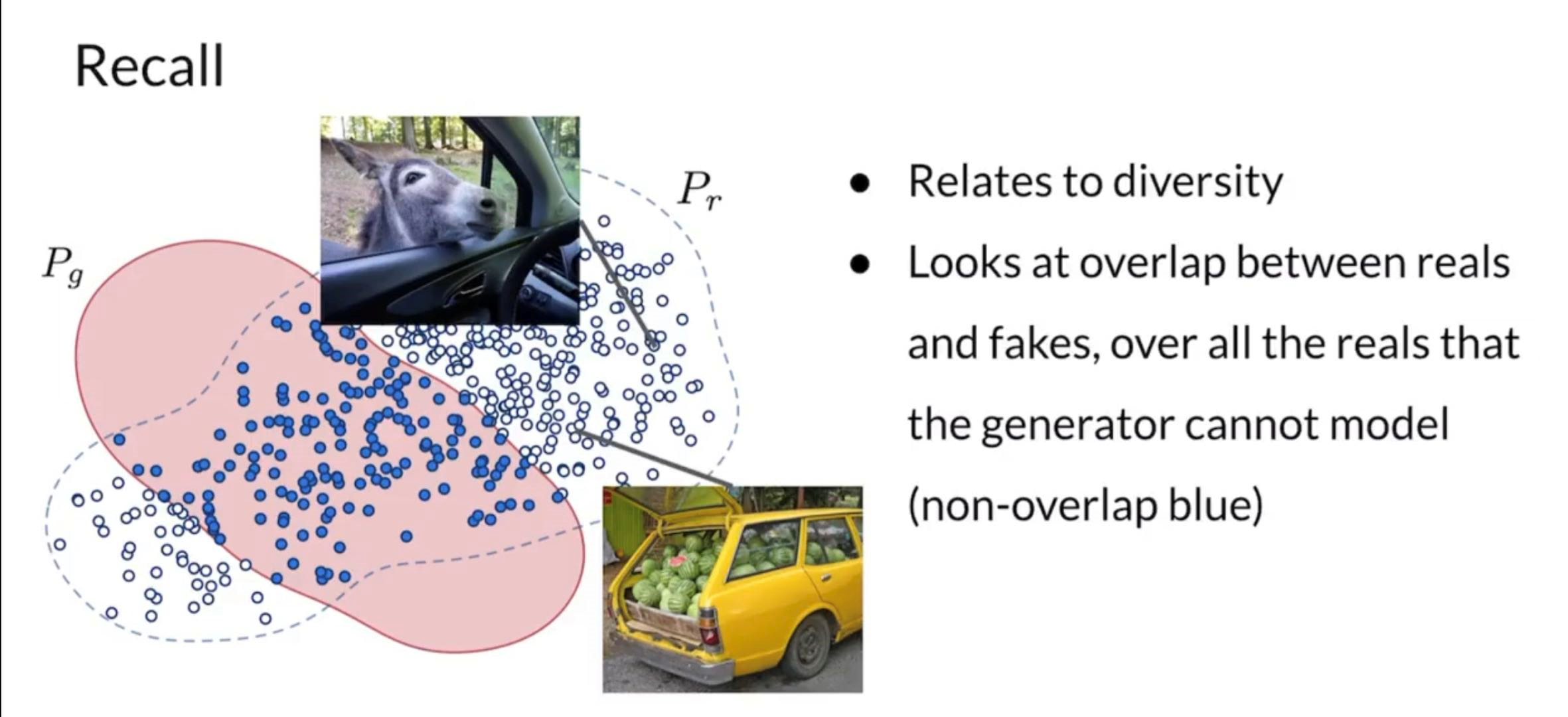
Recall: Area of real distribution overlapping with the fake distribution divded by area of real distribution. Percentage of real that can actually be faked ⇒ diversity of generated fakes

Models tend to be better at recall ⇒ but we can control precision by using truncation methods.

Shortcomings of GANs

1. Lack of Intrinsic Evaluation Metrics
   1. Even with FID distance its not ALWAYS reliable

2. Unstable training
   1. mode collapse
   2. is pretty much solved today
      1. by enforcing 1-L continuity through Wassertain Loss + Gradient Penalty, Spectral Norm
      2. by Instead of using generator model weights of a certain iteration count $\theta_i$, use a weighted average of weights at different iterations $\hat{\theta} = \frac{1}{n} \sum_{j=1}^n \theta_j$, this helps to smooth out generation.
      3. progressive growing
         1. see StyleGAN
   3. No density estimation for generated images
      1. Cannot do anomoly detection
   4. Inverting is not straightforward
      1. feed an image and find associated noise vector
      2. important for image editing

Because of those shortcomings, we will learn some alternatives to GANs (but will have tradeoffs)

Alternatives to GANs

Variational Autoencoders (VAE)

Has two parts encoder and decoder

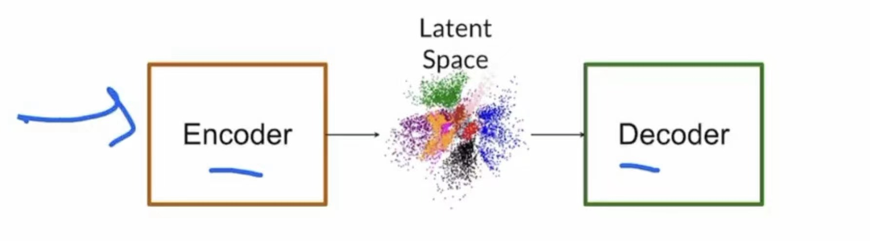
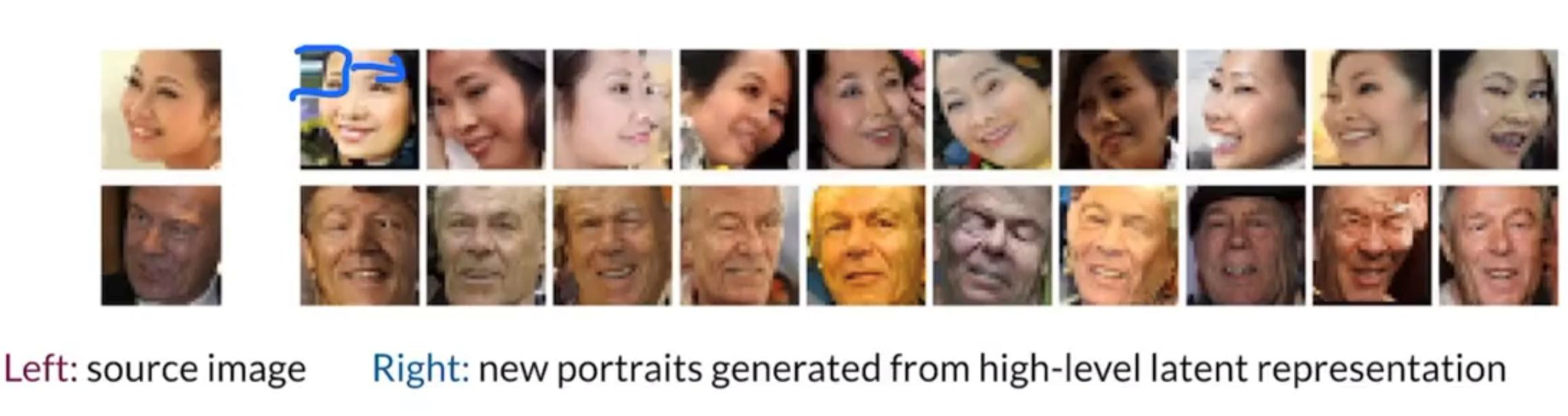
Encoder takes in images and translates it into a vector in latent space

Decoder takes in a latent space vector and spits out an image

minimizing the divergence between the input and the output, and only uses decoder portion during production.

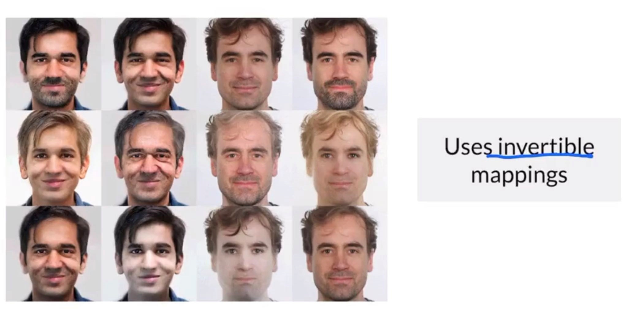
1. Has a density estimation

2. Operation is invertible

3. Has more stable training since the optimization problem of VAEs are easier

4. but produces lower quality results
   1. Lot of work put in to make result better

Autoregressive Models

Looks at previous pixels to generate new pixels fro a latent representation. It is supervised because it requires some pixels to be present first before it can generate.

FLOW models (Example: Glow)

Hybrid Models

e.g. VQ-VAE combines Autoregressive Model with VAE model.

Machine Bias

Machine Bias

On a spring afternoon in 2014, Brisha Borden was running late to pick up her god-sister from school when she spotted an unlocked kid's blue Huffy bicycle and a silver Razor scooter. Borden and a friend grabbed the bike and scooter and tried to ride them down the street in the Fort Lauderdale suburb of Coral Springs.

https://www.propublica.org/article/machine-bias-risk-assessments-in-criminal-sentencing

Machine Bias affects lives and we should be aware of those issues.

Defining Fairness

How to concretely measure how “fair” your model is?

1. Demographics parity
   1. Overall predicted distributions should be the same for different classes

2. Outcome that is a representation of actual demographics

3. Equality of Odds
   1. Make False Positive, False Negative EQUAL across classes

Ways Bias enter into models

1. training data
   1. no variation in data
   2. how data is collected
   3. diversity of the labellers
   4. “correctness” in culture
      1. side of the driver in the car

2. coders who designed the architecture

StyleGAN

Goals:

1. Greater fidelity on high-resolution images

2. Increased diversity of outputs

3. More control over image features

4. Tried both W-Loss and original GAN loss but found each one worked well with different dataset

5. Style can be any variation in the image, from high level to low level.

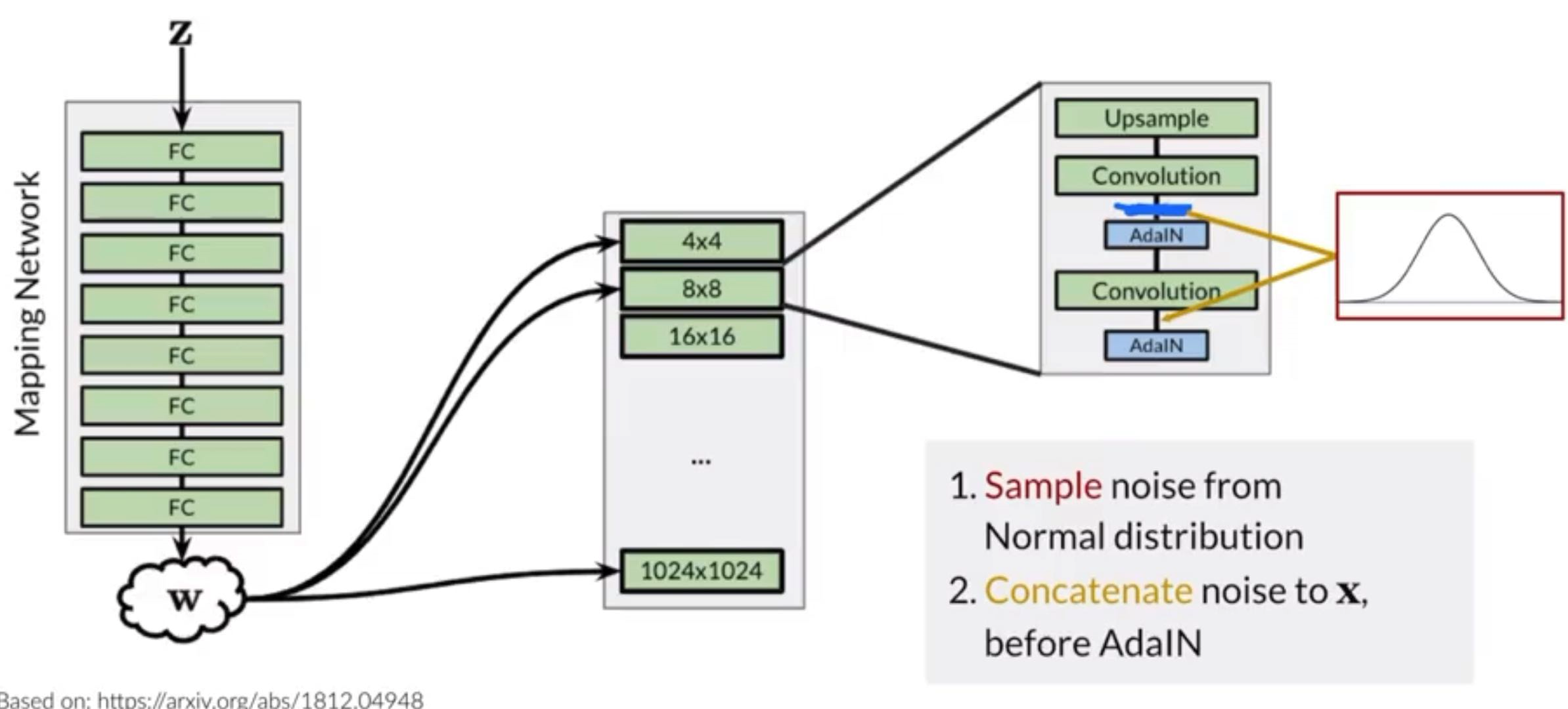
Basic Introduction

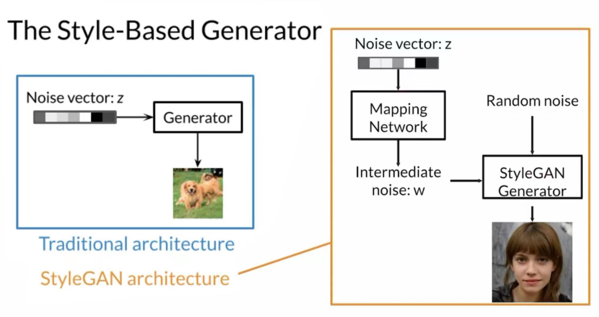
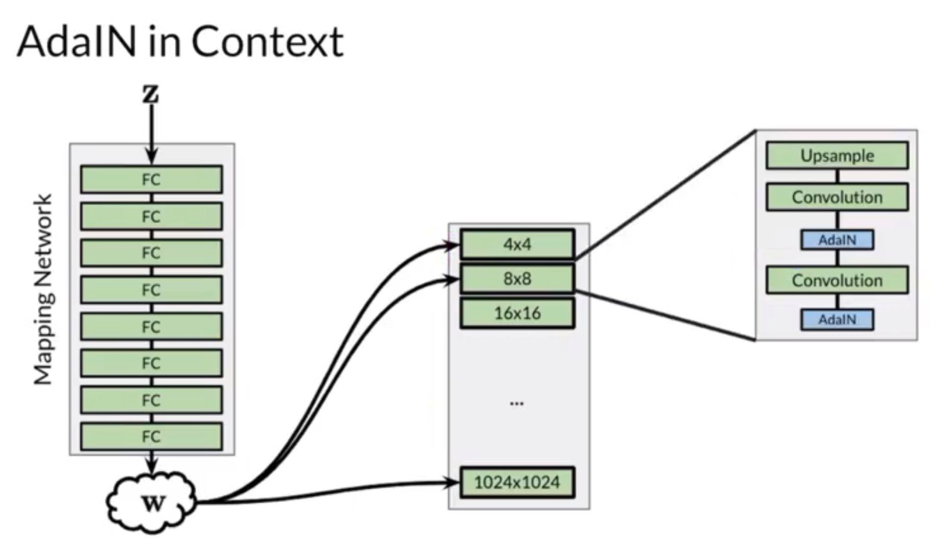
The $w$ noise is injected multiple times into the StyleGAN Generator through a technique called AdaIN(Adaptive Instance Normalization)

Random noise is added to increase the variance of the generated image

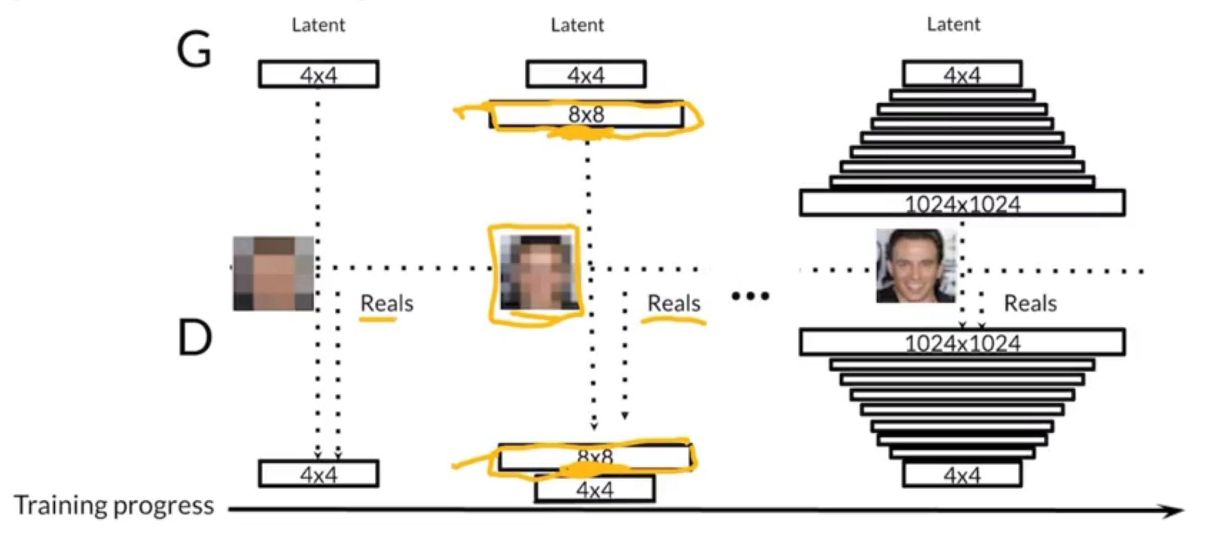
Progressive Growing

Idea: Easier to generate blurry faces and keep growing

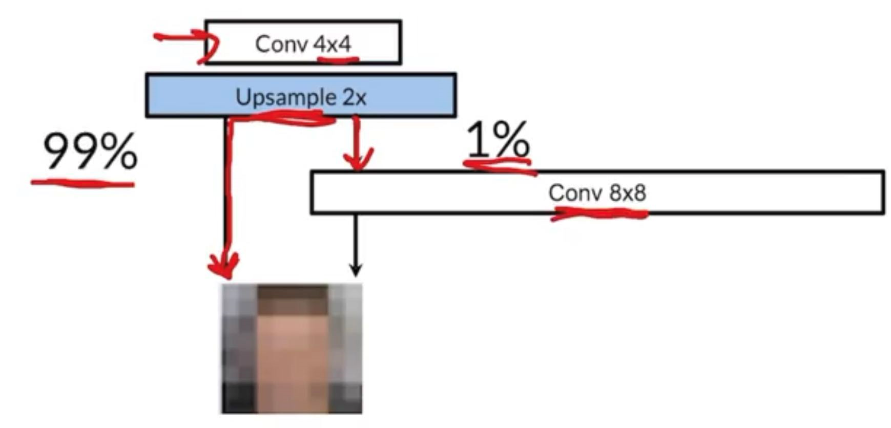
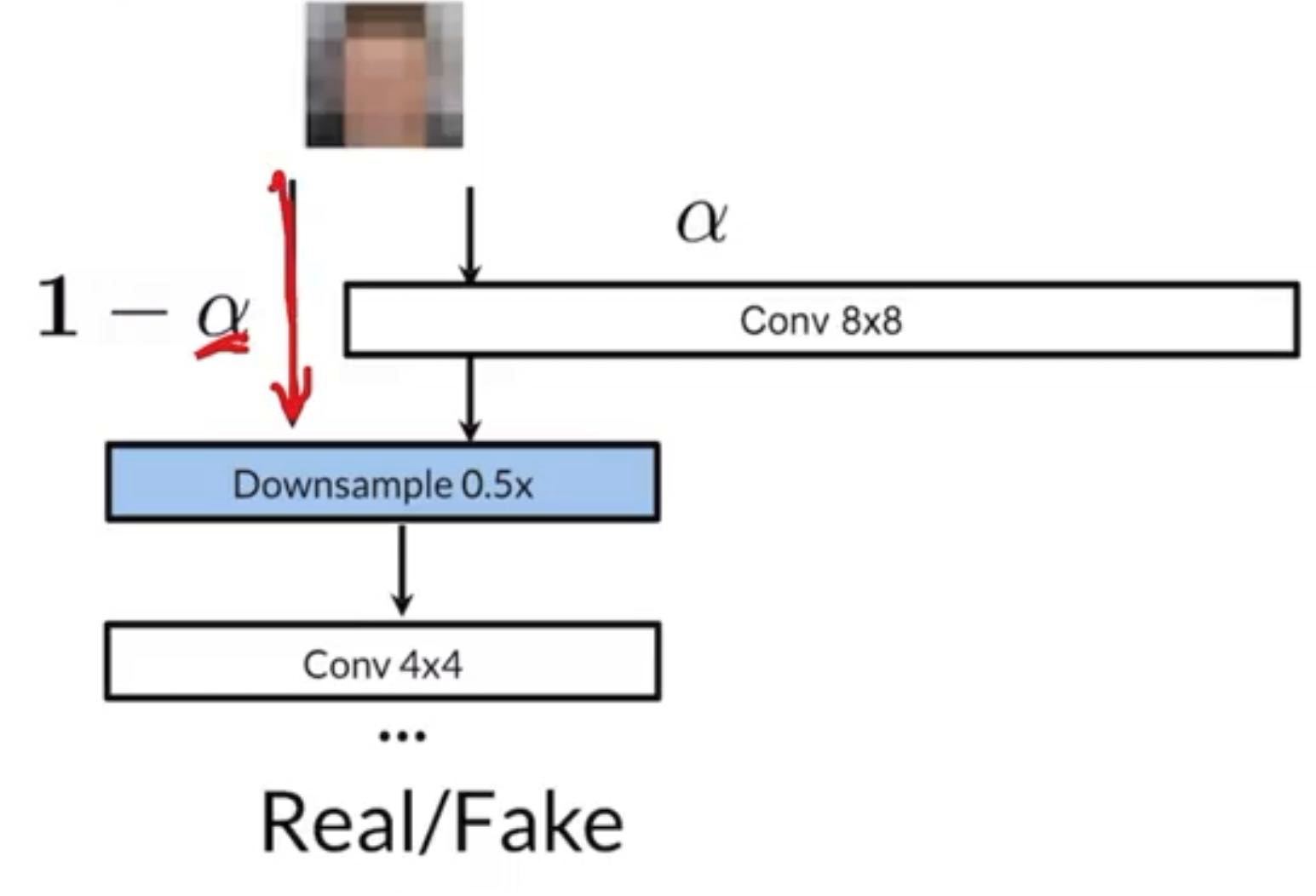
Say we want to grow the output of the generator from $4 \times 4$ to $8 \times 8$, we would put an upsample layer to the previous $4 \times 4$ output and the upsample layer then be followed by 99% nearest neighbour interpolation and 1% convolution. We will be able to learn some parameters for the new convolution layer. As time goes on, the percentage owned by the convolution layer would be tuned manually bigger and bigger (until we completely throw away the NN algorithm).

The percentage owned by the transpose convolution layer will be described by $\alpha$, and the percentage owned by NN algorithm would be $1 - \alpha$

(Pretty much same idea for discriminator)

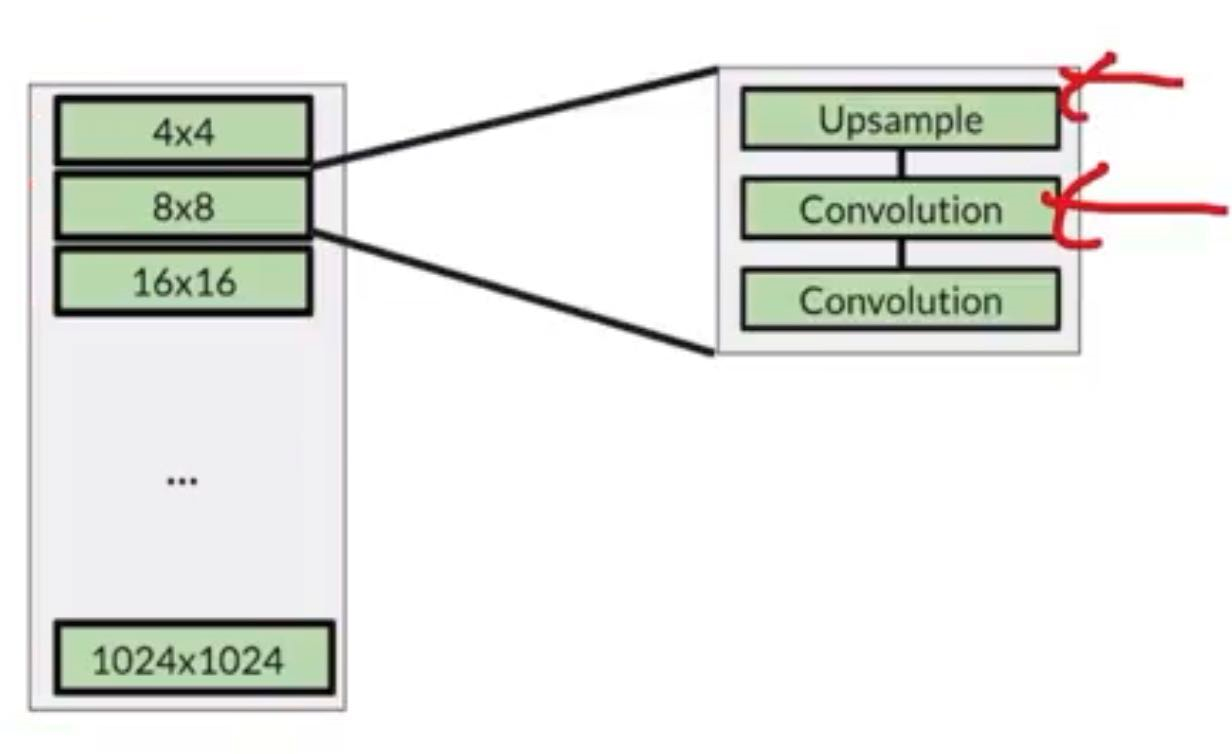
So Progressive Growing in StyleGAN looks like this in the architecture

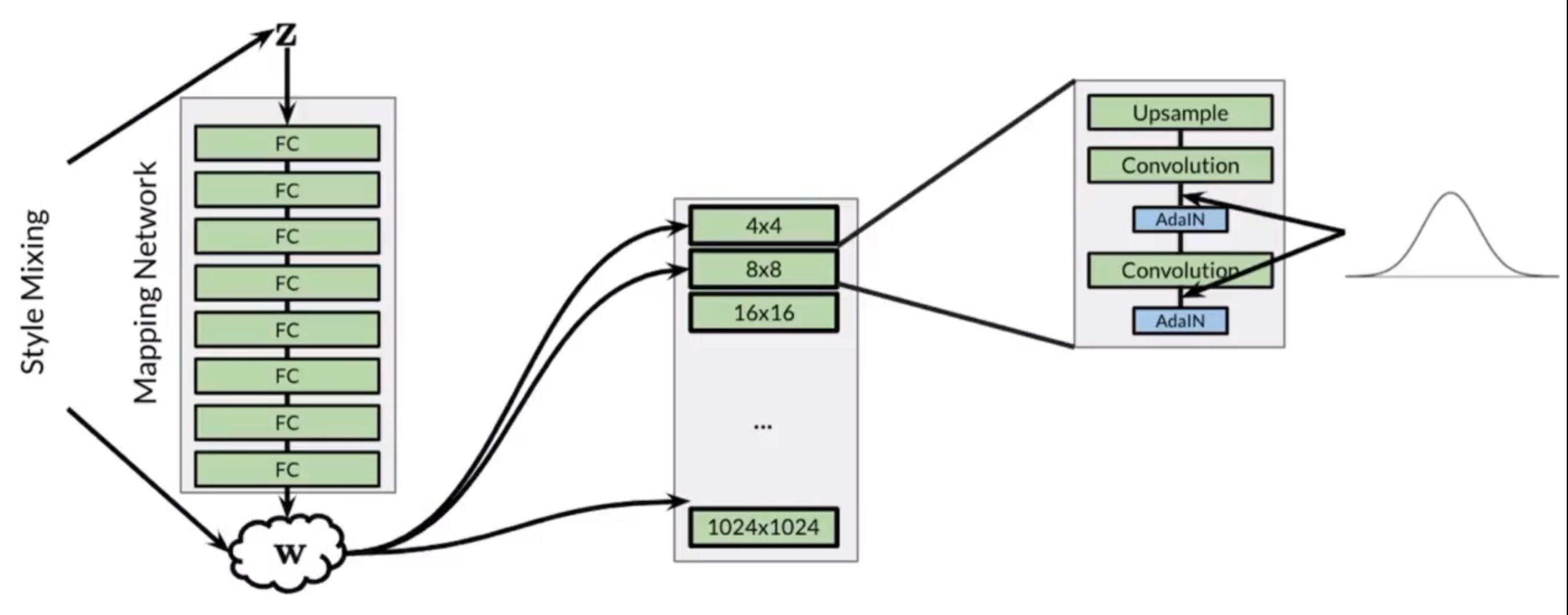
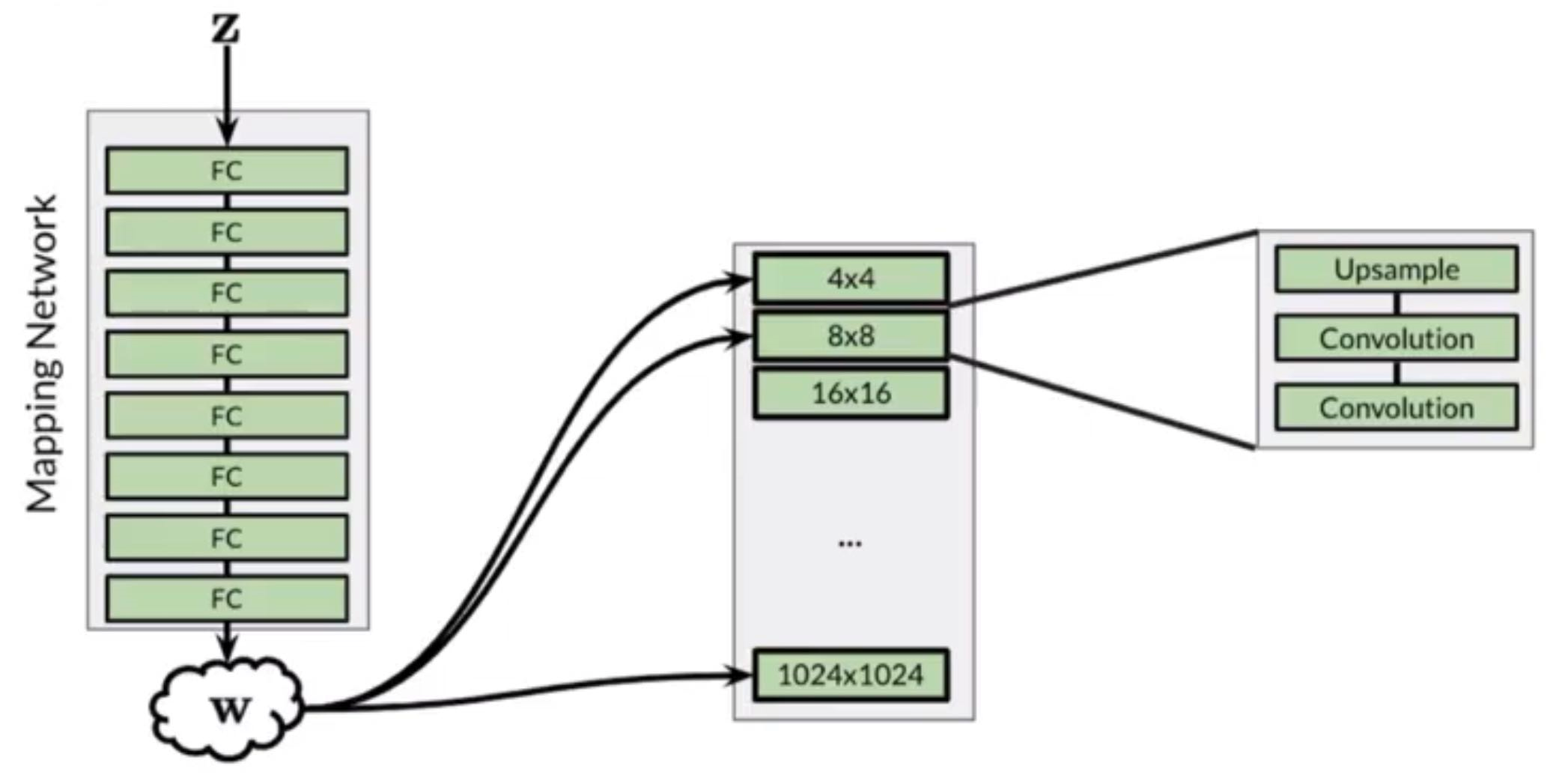
Noise Mapping Network

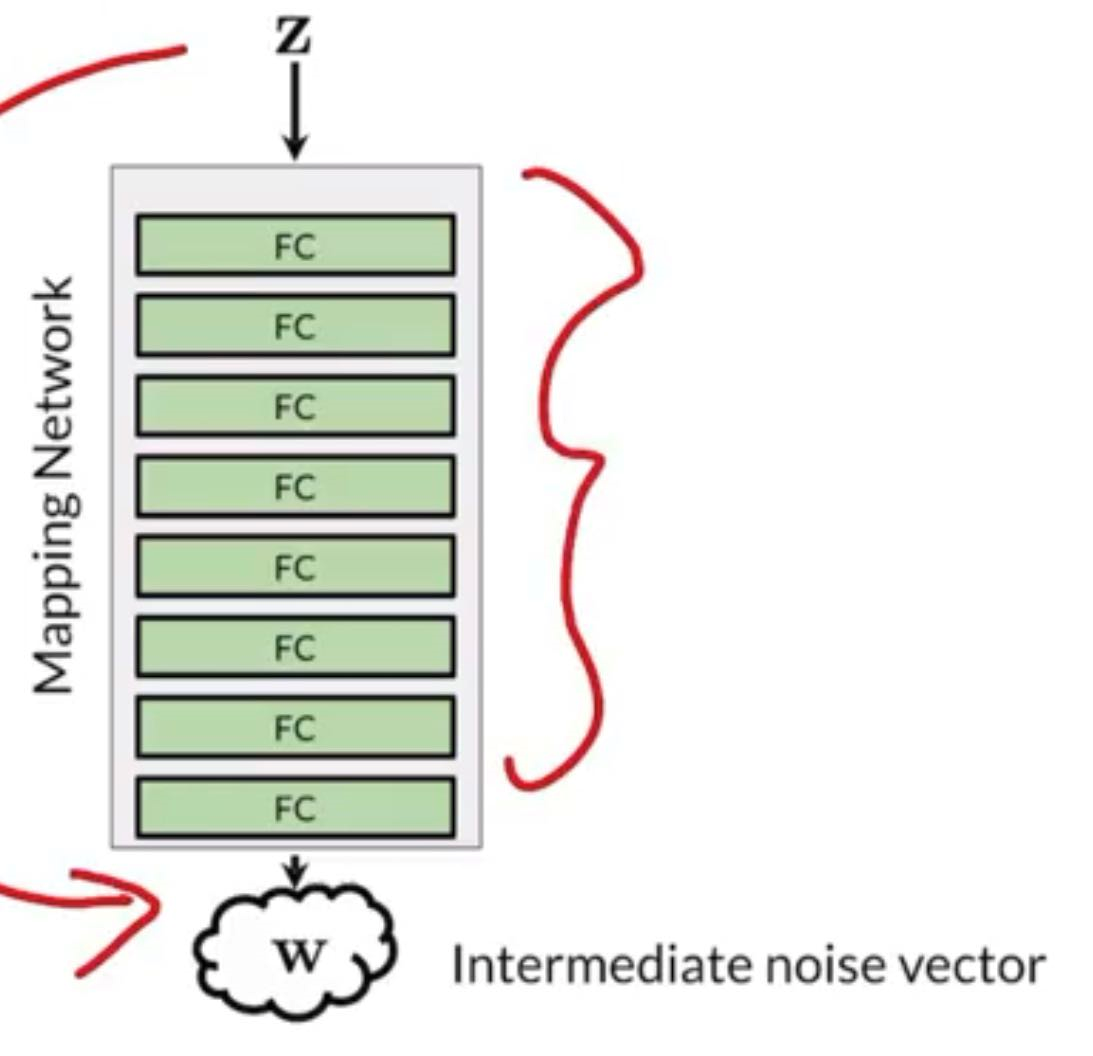
8-Layer MLP ⇒ 512 inputs and 512 outputs

Motivation: Mapping z to w helps disentangle noise representation

Probability Distribution of features have certain density, but z has normal prior, it is hard for z to be mapped to exact space of features.

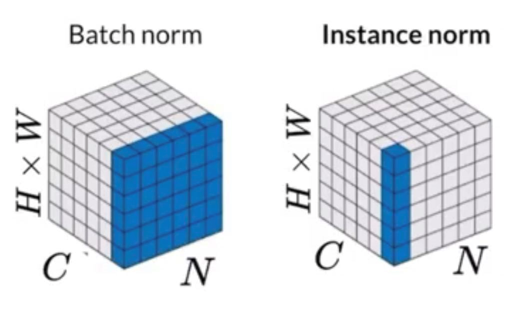
AdaIN (Adaptive Instance Normalization)

Instance Normalization

AdaIN

Apply Adaptive Styles using the intermediate noise vector $w$

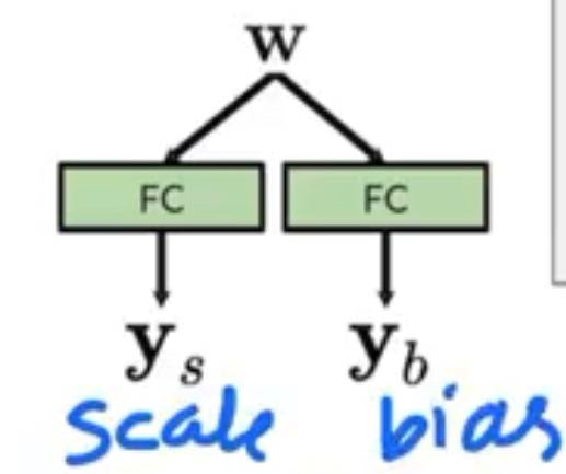
w is first inputted into two fully-connected layers (adaptive since the weights of those FC layers can change) to produce $y_s$ and $y_b$ which stands for scale and b, and then

The fraction part is basically just instance norm

Style Mixing

w is injected into all layers of the progressive growing layers, but we can actually inject different $z$ and therefore different $w$ into different parts of the network

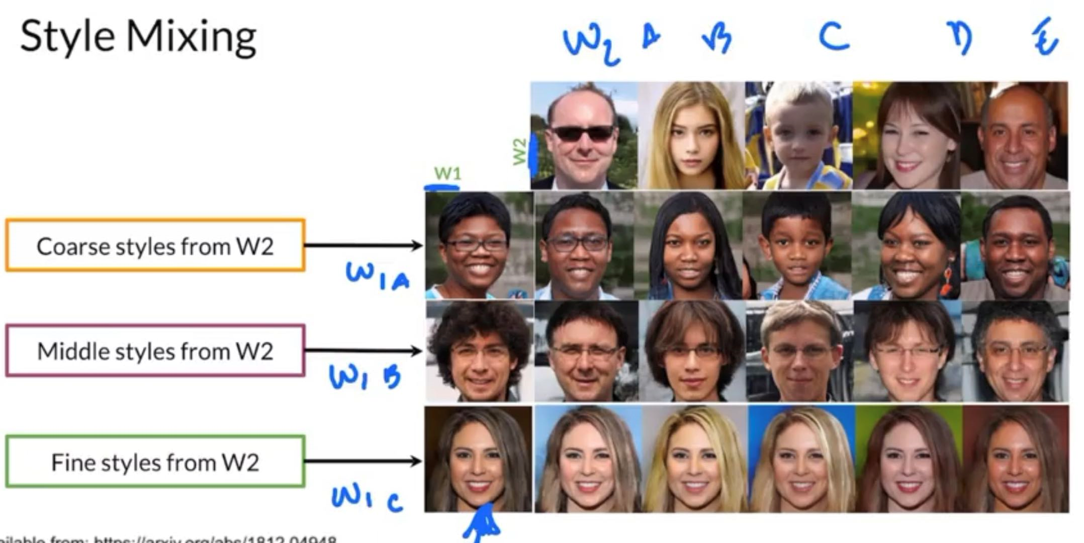
1. Can get more diversity in the things the model see in training

2. Can get control on granuity of details

Stochastic Variation

1. Don’t want mess of controlling two or more $w$ noises.

2. Can change very small details, like a very small piece of hair’s direction
   1. Have to inject in a deeper (or later) layer