P(A∣B) denotes the probability of event A happening when we know that event B is already happening.
P(A∣B)=1−P(A∣B)
P(A∣B)=P(B)P(A∩B)
P(A∣B)⋅P(B)=P(A∩B)
P(A)=P(A∣B)⋅P(B)+P(A∣B)⋅P(B)
Bayes’ Rule
P(A∣B)=P(B)P(B∣A)⋅P(A)
Counting & Sampling
Counting
Counting Sequence(Order Matters) Without Replacement
First Rule of Counting: If an object can be made by a succession of k choices, where there are n1 ways of making the first choice, and for every way of making the first choice there are n2 ways of making the second choice, and for every way of making the first and second choice there are n3 ways of making the third choice, and so on up to the nk-th choice, then the total number of distinct objects that can be made in this way is the product n1×n2×n3×⋯×nk.
nc=(N)k=(n−k)!n!
Counting Sequence With Replacement
nc=nk
Counting Sets without replacement
“n choose k”
nc=(kn)=(n−kn)=k!(N)k=(n−k)!k!n!
Second Rule of Counting: Assume an object is made by a succession of choices, and the order in which the choices are made does not matter. Let A be the set of ordered objects and let B be the set of unordered objects. If there exists an m-to-1 function f:A→B, we can count the number of ordered objects (pretending that the order matters) and divide by m (the number of ordered objects per unordered objects) to obtain ∣B∣, the number of unordered objects.
Counting Sets with replacement
Say you have unlimited quantities of apples, bananas and oranges. You want to select 5 pieces of fruit to make a fruit salad. How many ways are there to do this? In this example, S = {1, 2, 3}, where 1 represents apples, 2 represents bananas, and 3 represents oranges. k = 5 since we wish to select 5 pieces of fruit. Ordering does not matter; selecting an apple followed by a banana will lead to the same salad as a banana followed by an apple.
It may seem natural to apply the Second Rule of Counting because order does not matter. Let’s consider this method. We first pretend that order matters and observe the number of ordered objects is 35 as discussed above. How many ordered options are there for every un-ordered option? The problem is that this number differs depending on which unordered object we are considering. Let’s say the unordered object is an outcome with 5 bananas. There is only one such ordered outcome. But if we are considering 4 bananas and 1 apple, there are 5 such ordered outcomes (represented as 12222, 21222, 22122, 22212, 22221).
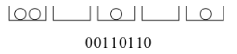
Assume we have one bin for each element of S, so n bins in total. For example, if we selected 2 apples and 1 banana, bin 1 would have 2 elements and bin 2 would have 1 element. In order to count the number of multisets, we need to count how many different ways there are to fill these bins with k elements. We don’t care about the order of the bins themselves, just how many of the k elements each bin contains. Let’s represent each of the k elements by a 0 in the binary string, and separations between bins by a 1.
Example of placement where |S| = 5 and k = 4
Counting the number of multisets is now equivalent to counting the number of placements of the k 0’s
The length of our binary string is k + n − 1, and we are choosing which k locations should contain 0’s. The remaining n − 1 locations will contain 1’s.
nc=(kn+k−1)
Zeroth Rule of Counting: If a set A can be placed into a one-to-one correspondance with a set B (i.e. you can find a bijection between the two — an invertible pair of maps that map elements of A to elements of B and vice-versa), then |A| = |B|.
Sampling
A population of N total, G good and B bad. sample size of n = g + b, with 0 ≤ g ≤ n
Sampling Sets with replacement
P(g good and b bad)=(gn)NnGgBb
Sampling Sets without replacement (Hypergeometric Dist.)
P(g good and b bad)=(gn)(N)n(G)g(B)b=(nN)(gG)(bB)
Probability Concepts
Consecutive Odds Ratios
Mainly used for binomial distribution
“Analyze the chance of k successes with respect to k-1 successes”
R(k)=P(k−1 successes)P(k successes)
Law of Large Numbers
As n→∞, the sampled mean will have a higher and higher probability of being in the actual distribution mean, P(∣n1Sn−μ∣<ϵ)→1, no matter how small ϵ is.
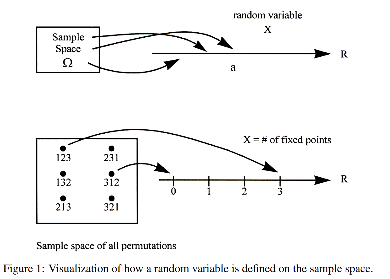
Random Variable
A random variable X on a sample space Ω is a function X:Ω→R that assigns to each sample point ω∈Ω a real number X(ω).
From CS70 Sp22 Notes 15
Probability of a value of a discrete random variable
P(X=x)=ω:X(ω)=x∑P(ω)
Has to satisfy:
∀x,P(X=x)≥0x∑P(X=x)=1
Note:
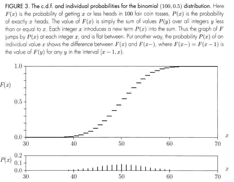
For discrete r.v., the CDF(cumulative distribution function) would be a step function
Probability of a value of a continuous random variable
P(X=x)=0
Probability of a range of value of a continuous random variable
P(a<X<b)=∫abf(x)dx
Has to satisfy:
∫−∞∞f(x)dx=1∀x,f(x)≥0
Continuous Random Variable
For continuous r.v.
There’s a Probability Density Function(PDF) and a Cumulative Distribution Function(CDF)
PDF: f(x)∀x,f(x)≥0 and ∫−∞∞f(x)dx=1
CDF: F(x)=P(X<x)=∫−∞xf(x)dxx→−∞limF(x)=0 and x→∞limF(x)=1
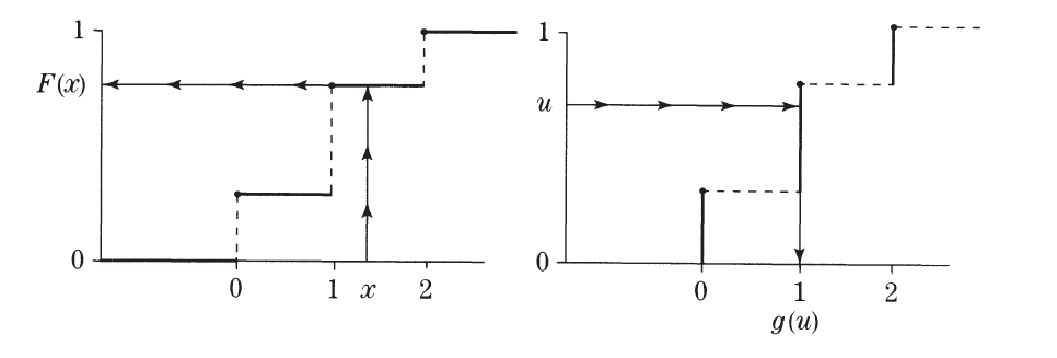
Inverse Distribution Function
For what value of x is there probability 1/2 that X ≤ x?
x=F−1(p)
Either calculate the inverse function of F(x) or solve equation F(x)=p, treating p as the variable.
Inverse CDF applied to standard norm
For any cumulative distribution function with inverse function F−1, if U has uniform (0,1) distribution, then F−1(U) has shape of CDF F(x).
Simulating binomial(n=2,p=0.5) with uniform distribution. g(u) here is equivalent to F(x) while g(U) here is equivalent to X
Probability Distribution
The distribution of a discrete random variable X is the collection of values {(a,P[X=a]):a∈A}, where A is the set of all possible values taken by X.
The distribution of a continuous random variable X is defined by its Probability Density Function f(x).
Example, For a dice, where X denotes the number on the dice when we roll the dice once.
P(X=1)=P(X=2)=P(X=3)=P(X=4)=P(X=5)=P(X=6)=61
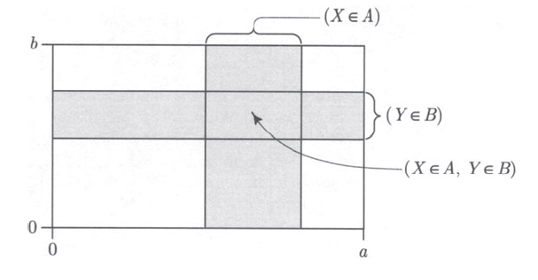
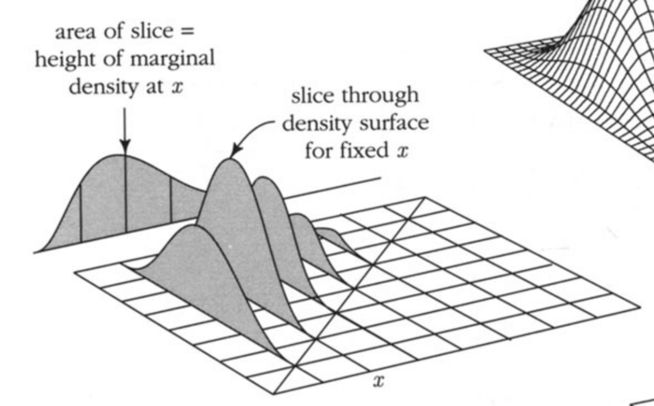
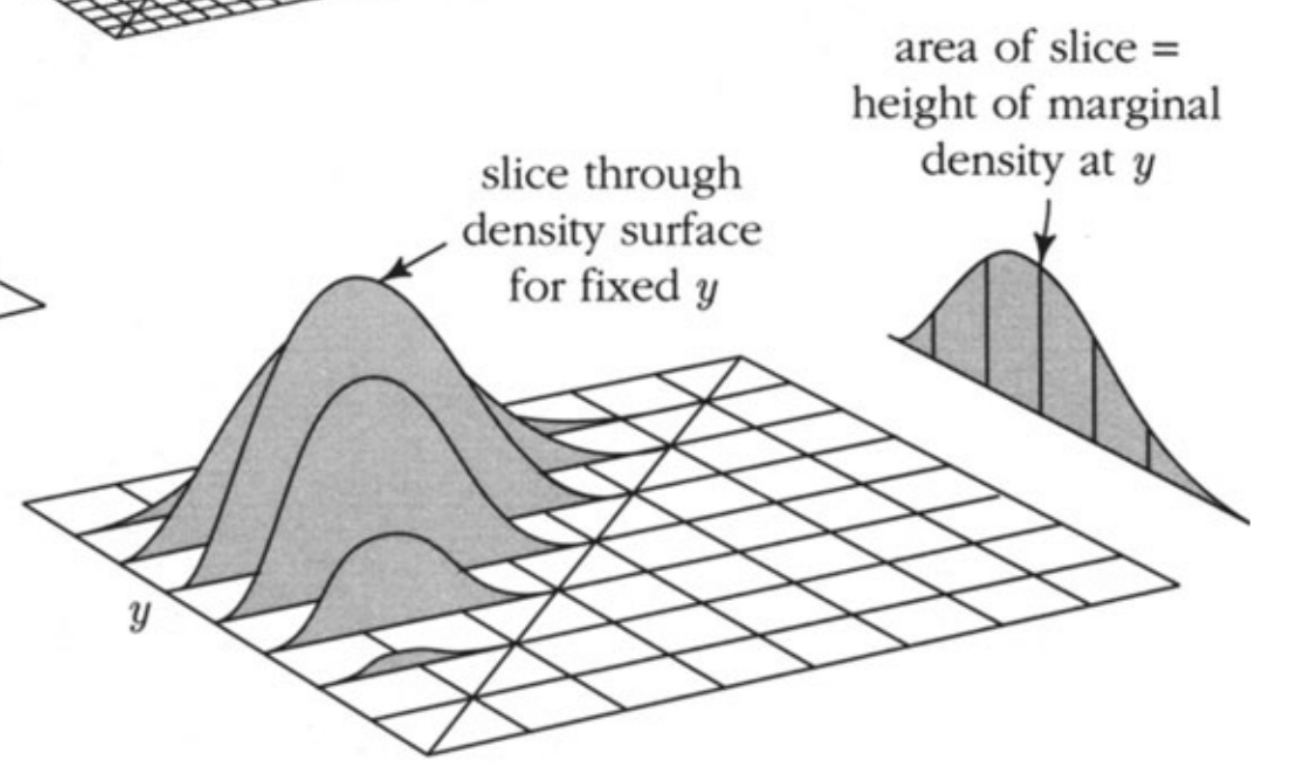
Joint Distribution
The joint distribution for two discrete random variables X and Y is the collection of values {(∀(a,b),P[X=a,Y=b]):a∈A,b∈B}, where A is the set of all possible values taken by X and B is the set of all possible values taken by Y
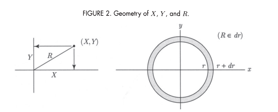
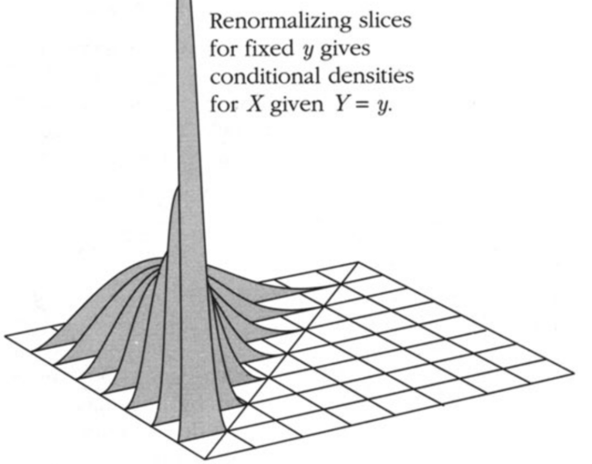
And the joint distribution for two continuous random variables X and Y is defined by the joint probabilty density function f(x,y). It gives the density of probability per unit area for values of (X,Y) near the point (x,y). P(X∈dx,Y∈dy)=f(x,y)dxdy.
In other words, list all probabilities of all posible X and Ys.
Has to satify the following constraint:
∀(a,b),P(X=a,Y=b)≥0a,b∑P(X=a,Y=b)=1
f(x,y)≥0∫−∞∞∫−∞∞f(x,y)dxdy=1
One useful equation:
P(X=a)=b∈B∑P(X=a,Y=b)
Symmetry of Joint Distribution
If X1,X2,…,Xn be random variables with joint distribution defined by
P(x1,x2,…,xn)=P(X1=x1,…,Xn=xn)
Then the joint distribution is symmetric if P(x1,…,xn) is a symmetric function of (x1,…,xn). In other words, for the value of P(x1,…,xn) is unchanged if we swap the positions of arbitrary number of parameters.
If the joint distribution is symmetric, then all n! possible orderings of the random variables X1,…,Xn have the same joint distribution and this means that X1,…,Xn are exchangeable. Exchangeable random variables have the same distribution.
Independence of random variables
Random variables X and Y on the same probability space are said to be independent if the events X=a and Y=b are independent for all values a, b. Equivalently, the joint distribution of independent r.v.’s decomposes as
X and Y has the same range, and for every possible value in the range,
∀v,P(X=v)=P(Y=v)
If X and Y has same distribution, then...
any statement of X has the same probability of the same statement of Y
g(X) has the same distribution with g(Y)
Combination of Random Variables
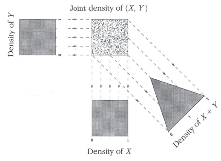
P(X+Y=k)=x∑P(X=x,Y=k−x)
fz(z)dz=∫xfx(x,z−x)dxdydy=dz since y=z−x
fz(z)=∫xfx(x)fy(z−x)dx
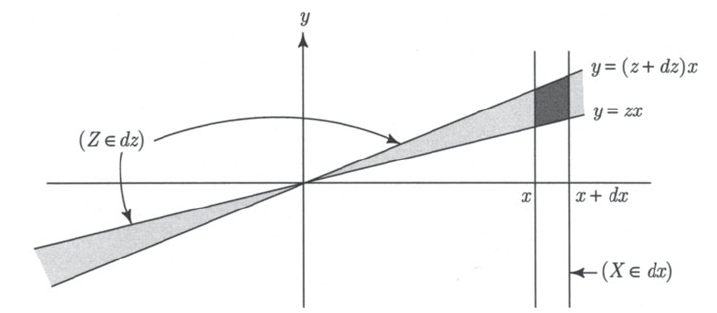
If Z=Y/X, Then Z∈dz is drawn in the following diagram
z=xy→y=zx
Note the area of the heavily shaded region here. It looks similar to a parallelogram. So area would be dx⋅[(z+dz)x−zx]=dxdz∣x∣.
P(X∈dx,Z∈dz)=f(x,xz)∣x∣dxdz
Therefore, if we integrate out X,
fz(z)=∫xf(x,xz)∣x∣dx
🙄
If X and Y are independent positive random variables, fz(z)=0(z≤0).
Equality of random variables
P(X=Y)=1⇔X=Y
“Equality implies identical distribution”
X=Y⟹∀v,P(X=v)=P(Y=v)
Probability of Events of two Random Variables
P(X<Y)=(x,y):x<y∑P(x,y)=x∑y:y>x∑P(x,y)
P(X=Y)=(x,y):x=y∑P(x,y)=x∑P(X=x,Y=x)
Symmetry of R.V.
The random variable X said to be symmetric around 0 if:
P(X=−x)=P(X=x)⇔-X has the same distribution as X⇔P(X≥a)=P(−X≤−a)=P(X≤−a)
Linear Function Mapping of Continuous Random Variable
suppose Y=aX+b and X has PDF fX(x)
then Y has PDF fY(y)=∣a∣1fX(ay−b)
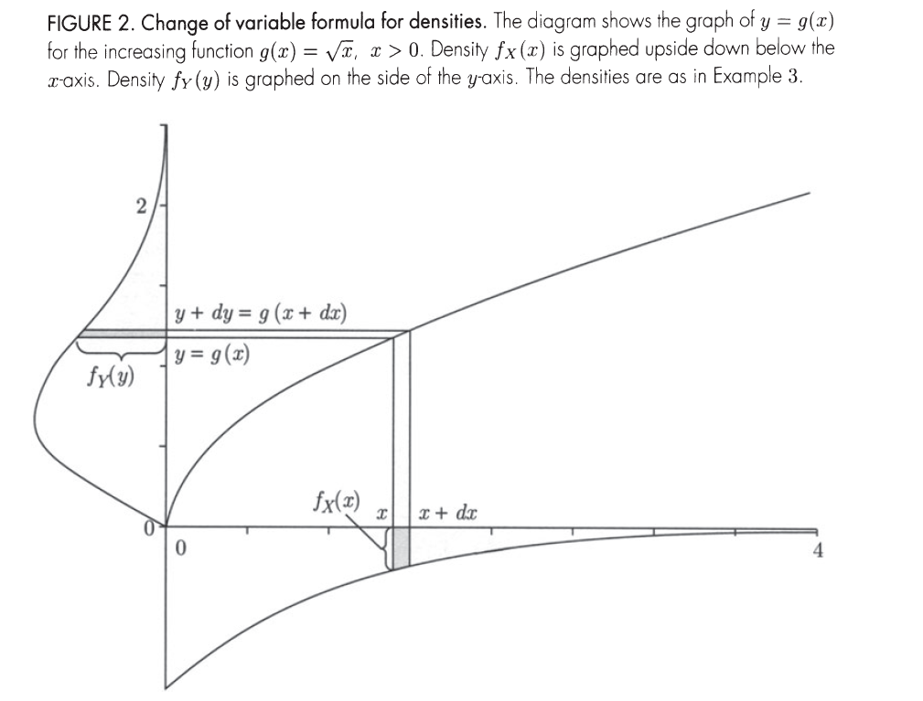
One-to-one Differentiable Function of Continuous Random Variable
Let X be a r.v. with density fX(x) on the range (a,b). Let Y=g(x) where g is strictly increasing or decreasing on interval (a,b).
For an infinitestimal interval dy near y, the event Y∈dy is identical to the event X∈dx.
Thus fY(y)∣dy∣=fX(x)∣dx∣. The absolute values are added in because for a decreasing function g(x), only the ratio of the magnitudes of dx and dy matters, thus:
fY(y)=∣dxdy∣fX(x)
Change of Variable Principle
If X has the same distribution as Y, then g(X) has the same distribution as g(Y), for any function g(⋅)
We use variance (squared error) instead of absolute error, E(∣X−μx∣), because it is easier to calculate
Variance of the sum of n variables
Var(k∑Xk)=k∑Var(Xk)+2j<k∑Cov(Xj,Xk)
Coefficient Property
Var(cX+b)=c2Var(X),where b,c∈R
Independent R.V. Variance
For Independent R.V. X,Y, we have:
Var(X+Y)=Var(X)+Var(Y)
Standard Deviation σ
σx=Var(X)
Standardizations of Random Variable
X∗=σX−μx
“X in standard units” with E(X∗)=0,Var(X)=σx=1
Skewness of R.V.
Let X be a random variable with E(X)=μ and Var(X)=σx2, Let X∗=σX−μ be X in standard units.
Skewness(X)=E[(X∗)3]=σ3E[(X−μ)3]
Markov’s Inequality
Note: For nonnegative R.V.s only
If X≥0,P(X>a)≤aE(X)
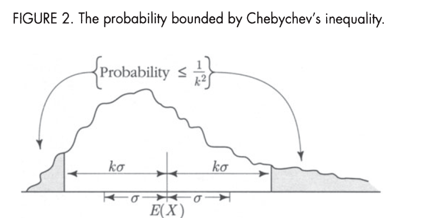
Chebychev’s Inequality
P(∣X−E(X)∣≥kσx)≤k21P(∣X−μ∣≥c)≤c2Var(X)
Order Statistics
Let X1,X2,X3,…,Xn be random variables with the independent and identical distribution pdf f(x) and cdf F(x)
Then if we denote X(1),X(2),…,X(n) being the smallest, the second smallest, etc. among X1,…,Xn. Then what is the distribution of X(i)?
f(k)(x)dx=P(X(k)∈dx)=P(one of the X’s∈dx,exactly k−1 of others <x=nP(X1∈dx,exactly k−1 of others <x)=nP(X1∈dx)P(exactly k−1 of others <x)=nf(x)dx(k−1n−1)(F(x))k−1(1−F(x))n−k(−∞<x<∞)
If correlation is equal to ±1, it means the two variables have linear relationship. For details, see the proof above.
Moment Generating Function
Let X be a random variable, then the MGF(Moment Generating Function) of X is defined as
MX(t)=E(etX)
Important Properties
Equality of MGF means Equality of CDF
MX(t)=MY(t)⟹FX(x)=FY(x)
Jensen’s Inequality
MX(t)≥eμt,μ=E(X)
Upper tail of random variable using Markov’s Inequality
P(X≥a)=P(etX≥eta)≤etaE(etX)=e−taMX(t)
Linear Transformation of Random Variable
MαX+β(t)=E(eαtX+βt)=eβtE(eαtX)=eβtMX(αt)
Linear Combination of Independent Random Variables
M∑i=1naiXi(t)=i=0∏nMXi(ait)
Additional Topic - MLE and MAP
💡
Maximum Likelihood Estimation and Maximum A Posteriori are two topics that I personally got confused by during the study of CS189. So here I will give links to some great videos and a little bit mathematical formulas for MAP and MLE.
Say we have observations x, we want to estimate a parameter θ, where θ is a random variable.
MLE does the following:
θMLE=θargmaxP(x∣θ)
MAP does the following:
θMAP=θargmaxP(θ∣x)
💡
We see that MLE maximizes the likelihood of having the observations given the parameter, while MAP maximizes the posterior probability of having the parameter giving the observation.
MLE - iterate through distribution parameters and find the distribution parameter such that producing x is most likely using the parameter.
MAP - iterate through distribution parameters and find the distribution parameter that is most likely to be right given the observed data.
By Bayes Theorem,
P(θ∣x)=P(x)P(x∣θ)P(θ)
Note that
P(x)=E(P(x∣θ))=∫θf(x∣θ)f(θ)dθ
Since P(x) is independent of individual θ, we can view P(x) as a constant, and therefore,
P(θ∣x)∝P(x∣θ)P(θ)=P(x,θ)
Therefore, MAP can also be written as
θMAP=θargmaxP(θ∣x)=θargmaxP(x∣θ)P(θ)
💡
See the difference between the term optimized by MAP and MLE here? The MAP has an addition of P(θ). If the prior, P(θ) is the same across all θ (uniform prior distribution), then MAP is identical with MLE.
Properties of MLE and MAP
Note that both MLE and MAP are point estimators, that is if the parameter is continuous (and usually this is the case), then it picks the max point on the PDF function, not the midpoint of the points where their areas are the biggest.
MLE is more prune to overfitting then MAP, since the prior in MAP kind of restricts the parameter estimated in an area.
the asymptotic behavior of MAP and MLE are the same, that is as we collect more data, the result of MAP and MLE tends to converge.
Special Property of MLE (not applicable to MAP): T=g(θ)⟹TMLE=g(θMLE)
Distribution
Bernoulli(Indicator) Distribution In∼Bernoulli(p)
P(In=1)=pP(In=0)=1−p
E(In)=p
Var(In)=p(1−p)
Uniform Distribution on a finite set
Let we have a list of uniform events, Ω={ω1,ω2,…,ωn}
∀i,P(ωi)=n1
Uniform(a,b) distribution
Distribution of a point picked uniformly at random from the interval (a,b)
For a < x < y < b the probability that a point falls in the interval (x,y) is...
P(a<x<y)=b−ay−x
for b-a= 1, long-run frequency is almost exactly equal to y-x.
PDF: f(x)={b−a10if a<x<botherwise
Empirical Distribution
Opposed to theoretical distribution, empirical distribution is the distribution of your observed data.
Suppose we have X={x1,x2,…,xn}
Pn(a,b)=n∣i:1≤i≤n,a<xi<b∣
In other words, Pn(a,b) gives the proportion of the numbers in the list that lies in-between range of (a,b)
Estimating Empirical Distribution With Continuous PDF
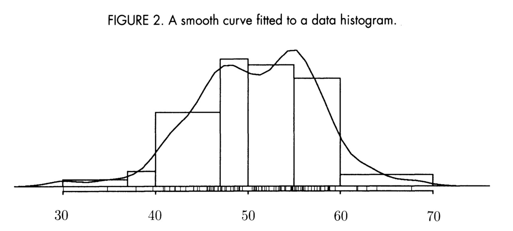
The distribution of a data list can be displayed in a histogram, and such histogram smoothes out the data to display the general shape of the empirical distribution.
Such histograms often follows a smooth curve f(x). And it is safe to assume ∀x,f(x)≥0
Idea is that if (a,b) is a bin interval, then the area under the bar between (a,b) should roughly equal to the area under the curve between (a,b) ⇒ the proportion of data from a to b is roughly equal to the area under f(x).
Pn(a,b)≈∫abf(x)dx
f(x) functions like a continuous PDF estimation for distribution of data.
Now we can also use an indicator distribution to estimate its average
I(a,b)(x)={10if x∈(a,b)otherwise
So I(a,b)(xi) is an indicator stating if xi is in range of (a,b)
If the empirical distribution of list (x1,x2,…,xn) is well approximated by the theoretical distribution with PDF f(x), then the average value of a function g(x) over the n values can be approximated by
n1i=1∑ng(xi)≈∫−∞∞g(x)f(x)dx
Binomial Distribution X∼B(n,p)
“probability of k successes in n trials with success rate of p”
P(X=k)=(kn)pk(1−p)n−k
R(k)=[kn−k+1]1−pp
E(X)=npVar(X)=np(1−p)
Note: “Binomial Expansion”
(p+q)n=k=0∑n(kn)pkqn−k
Square Root Law
For large n, in n independent trials with probability p of success on each trial:
the number of success will, with high probability, lie in a ralatively small region centered on np, with width a moderate multiple of n on the numerical scale
the proportion of success will, with high probability, lie in a small interval centered on p, with width a moderate multiple of n1
Normal Distribution as an approximation for Binomial Distribution
👉
Used when p≈21
provided n is large enough in X∼B(n,p), X can be approximated with normal distribution
If approximating a to b success in a bionomial distribution, use b+21 and a−21 as the boundary instead of using b and a, this is called continuity correction. Very important for small values of npq.
P(a≤X≤b)≈Φ(b+21)−Φ(a−21)
Note: for f(x), use μ=E(X) and σ2=Var(X) of the Binomial distribution
👉
How good is the normal distribution? Its best when σ=npq is big and p is close to 21
W(n,p)=0≤a≤b≤nmax∣P(a to b)−N(a to b)∣≈101npq∣1−2p∣
W(n,p) denotes the WORST ERROR in the normal approximation to the binomial distribution.
Poisson Distribution as an approximation for binomial distribution
When n is large and p is close to 0, normal distribution cannot properly estimate binomial distribution, so let’s use poisson! (if p is close to one, use the p = original q and mirror the approximation to get the approximation)
X∼B(n,p)∼Poisson(μ=np)
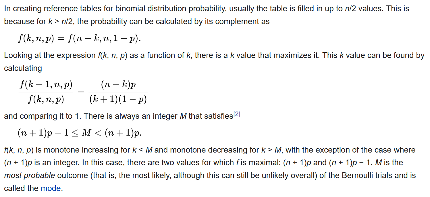
Probability of the Most Likely Number of Successes
Taken from wikipedia
m=⌊np+p⌋=⌈np+p−1⌉
P(m)∼2πσ1
Normal Distribution X∼N(μ,σ2)
PDF:f(x)=2πσ1e−21(σ(x−μ))2,−∞<x<∞
Standard Normal Distribution (μ=0,σ=1)
PDF:ϕ(z)=2π1e−21z2
CDF:Φ(z)=∫−∞zϕ(y)dy
Where z=σx−μ=x
Skew Normal Aproximation
“Third derivative of ϕ(z)”
ϕ′′′(z)=(3z−z3)ϕ(z)
“Skew-normal PDF”
ϕ(z)≈ϕ(z)−61Skewness(n,p)⋅ϕ′′′(z)
Skewness(n,p)=npq1−2p=σ1−2p
“Skew-normal CDF”
Φ(z)≈Φ(z)−61Skewness(X)⋅(z2−1)⋅ϕ(z)
“0 to b success rate” for binomial distribution
P(0 to b success)≈Φ(z)−61Skewness(n,p)⋅(z2−1)⋅ϕ(z)
where z=σb+21−μ,μ=np,σ=npq
Sum of Independent Normal Variables
If X∼N(λ,σ2) and Y∼N(μ,r2), then X+Y∼N(λ+μ,σ2+r2)
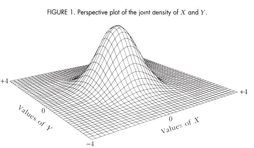
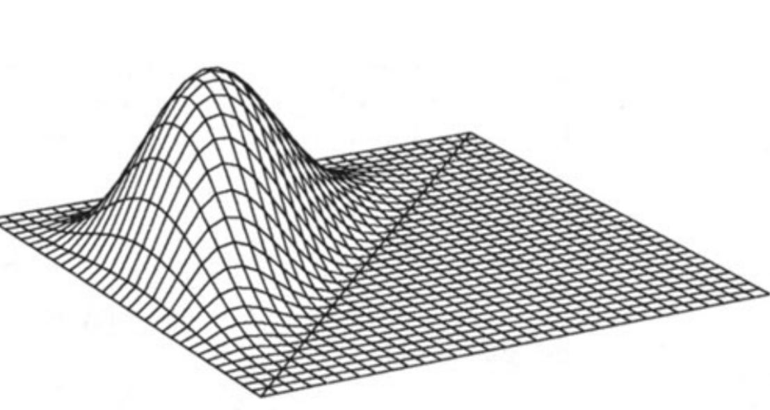
Joint Distribution for Independent Standard Normal Distributions
let X and Y be standard normal dist, that is X,Y∼N(μ=0,σ2=1)
ϕ(z)=ce−21z2(c=2π1)
f(x,y)=ϕ(x)ϕ(y)=c2e−21(x2+y2)
📎
Notice the rotational symmetry of this joint distribution.
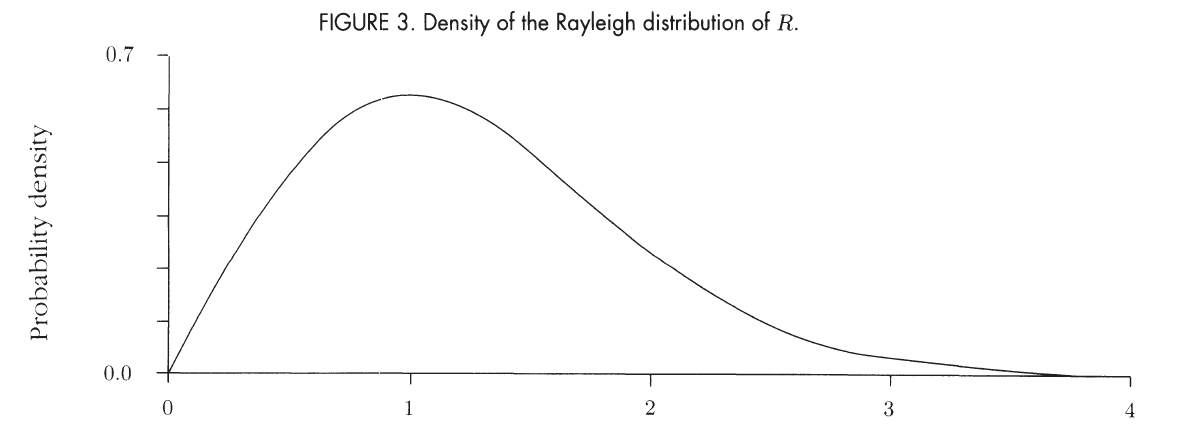
Rayleigh Distribution R∼Rayleigh
Its the distribution of the above joint distribution of standard normal distribution along the radius.
PDF: fR(r)=re−21r2(r>0)
CDF: FR(r)=∫0rse−21s2ds=1−e−21r2
E(R)=σ2π
Var(R)=24−πσ2
Derivation of Rayleigh Distribution
R=X2+Y2
ϕ(x,y)=c2e−21(x2+y2)=c2e−21r2
P(R∈dr)=2πr⋅dr⋅c2e−21r2
And therefore
fR(r)=2πrc2e−21r2
Notice that fR(r) must integrate to 1 over (−∞,∞), if we calculate this, we see that ∫0∞fR(r)dr=2πc2, and therefore c=1/2π.
Chi-Square Distribution
Joint density of n independent normal variables at every point on the sphere radius r in n-dimensional space is:
fR(r)=(2π1)nexp(−21r2)
For independent standard normal Zi, let the following denote the distance in n-dimensional space
Rn=Z12+⋯+Zn2
So the n-dimensional volumnof a thin spherical shell of thickness dr at radius r is
cnrn−1dr
Where cn is the (n-1) dimensional volumn of the “surface” of a sphere of radius 1 in n dimensions
c2=2π,c3=4π,…
P(Rn∈dr)=cnrn−1(1/2π)ne−21r2dr(r>0)
Through a change of variable and evaluating cn we see that the density of Rn2∼Gamma(r=n/2,λ=1/2).
We call Rn2 follows the distribution of the chi-square distribution with n degrees of freedom.
E(Rn2)=nVar(Rn2)=2n
Skewness(Rn2)=4/2n
Standard Bivariate Normal Distribution
X and Y have standard bivariate normal distribution with correlation ρ iff:
Y=ρX+1−ρ2Z
where X and Z are independent standard normal variables
Joint Density:
f(x,y)=2π1−ρ21exp{−2(1−ρ2)1(x2−2ρxy+y2)}
Properties:
Marginals
Both X and Y have standard normal distribution
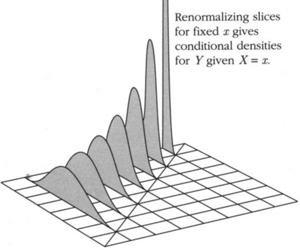
Conditionals Given X
Given X=x, Y∼N(ρx,1−ρ2).
Conditionals Given Y
Given Y=y, X∼N(ρy,1−ρ2)
Independence
X and Y are independent iff ρ=0
Bivariate Normal Distribution as a description for Linear Combinations of Independent Normal Variables
Let
V=i∑aiZi,W=i∑biZi
Where Zi∼N(μi,σi2) are independent normal variables.
Then the joint distribution of V,W is bivariate normal.
Two linear combinations V=∑iaiZi and W=∑ibiZi of independent
normal (μi,σi2) variables Zi are independent iff they are uncorrelated,
that is, if and only if ∑iaibiσi2=0.
Bivariate Normal Distribution
Random Variables U and V have bivariate normal distribution with parameters μU,μV,σU2,σV2,ρ iff the standardized variables
U∗=σUU−μU,V∗=σVV−μV
have standard bivariate normal distribution with correlation ρ. Then,
ρ=Corr(U∗,V∗)=Corr(U,V)
and U,V are independent iff ρ=0
Derivation
📎
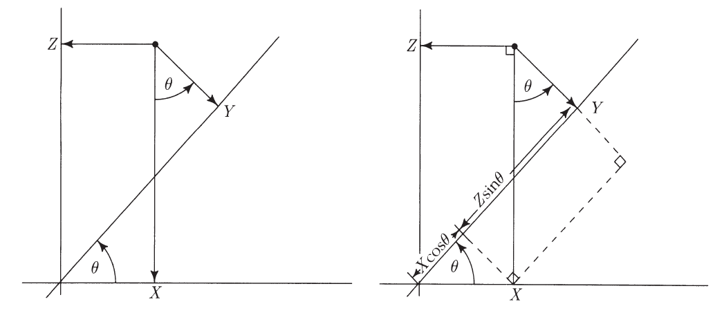
Goal: to construct a pair of correlated standard normal variables.
We start with a pair of independent standard normal variables, X and Z.
Let Y be the projection of (X,Z) onto an axis at an angle θ to the X-axis,
We see on the diagram that Y=Xcos(θ)+Zsin(θ)
By rotational symmetry of the joint distribution of X,Z, the distribution of Y is standard normal.
As μ starts small the distribution is piled up on the side and as λ gets bigger and bigger, the poisson distribution becomes closer to the normal distribution (theres a proof that n→∞,p=nλ→0, the approximation becomes better and better)
Sum of Independent Poisson Variables
N1,...,Nj are independent Poisson random variables with parameters μ1,...,μj, then S=N1+N2+⋯+Nj, S∼Poisson(∑i=1jμi)
Skew-normal approximation for Poisson Distribution
If Nμ∼Poisson(μ), then for b = 0, 1, ...
P(Nμ≤b)≈Φ(z)−6μ1(z2−1)ϕ(z)
where ϕ(z) is the standard normal curve and Φ(z) is the standard normal CDF.
Multinomial Distribution
“a generalization of the binomial distribution” ⇒ Bionmoial Distribution With Multiple Types of Outcomes(instead of 2)
Let Ni denote the number of results in category i in a sequence of independent trials with probability pi for a result in the ith category for each trial, 1≤i≤m, where ∑i=1mpi=1. Then for every m-tuple of non-negative integers (n1,n2,…,nm) with sum n:
For large n, the distribution of Sn is approximately normal, which means:
E(Sn)=nμxσ2(Sn)=nσx2Sn∼N(nμx,nσx2)
Note: To approximate Probability of Sn taking a specific range of values, we need to use continuity estimation(add and subtract 21×n on the upper and lower bound)
👉
Why 21×n instead of 21? Because nX can only take values that are multiples of n
For all a≤b,
P(a≤σnSn−nμx≤b)=Φ(b)−Φ(a)
👉
Sn∗, the “Sn in standard units”, equals to SD(Sn)Sn−E(Sn)=σnSn−nμx
Skewed-Normal Approximation
Φ(z)≈Φ(z)−6n1Skewness(Xi)ϕ(z)
Hypergeometric Distribution
This is also the section of “sampling without replacement”
P(g good and b bad)=(gn)(N)n(G)g(B)b=(nN)(gG)(bB)
P(Sn=g)=(nN)(gG)(bB)
where b=n−g
E(Sn)=npVar(Sn)=N−1N−n⋅npq
where p=NG and q=NB.
N−1N−n is the “finite population correction factor”
Exponential Distribution T∼Exponential(λ)
A random time T has exponential distribution with rate λ ⇒ probability of death per unit time
A positive random variable T has exponential(λ) distribution for some λ > 0 if and only if T has the memoryless property
P(T>t+s∣T>t)=P(T>s)(s≥0,t≥0)
“Given survival to time t, the chance of surviving a further time s is
the same as the chance of surviving to time s in the first place.”
Relation to Geometric Distribution
The exponential distribution on (0,∞) is the continuous analog of the geometric distribution on {1,2,3,…}
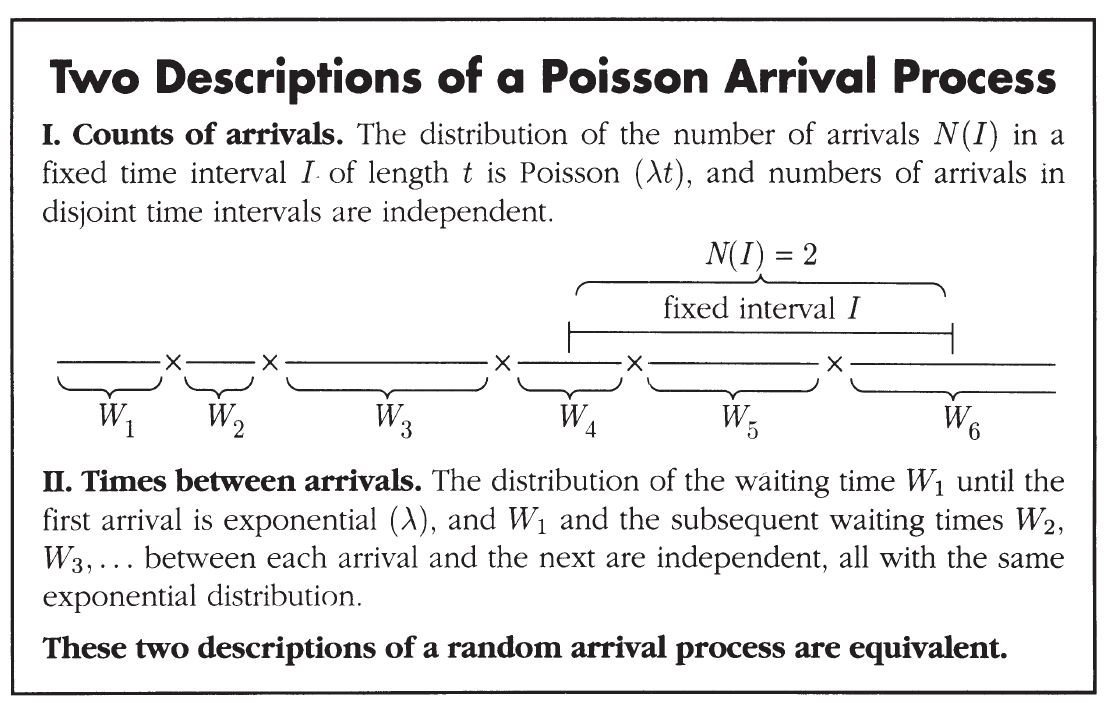
Relation to Poisson Arrival Process
A sequence of independent Bernoulli(Indicator) trials, with probability p of success on each trial, can be characterized in two ways:
Counts of successes - number of successes in n trials is Binomial(n,p)
Times between successes - distribution of the waiting time until the first success is Geometric(p), waiting times between each successes and the next are independent with the same geometric distribution.
These characterization of Bernoulli trials lead to the two descriptions in the next box of a Poisson Arrival Process With Rate λ.
👉
Arrivals are at times marked with X on the time line, think of arrivals representing something like incoming calls or customers entering a store
Gamma Distribution Tr∼Gamma(r,λ)
If Tr is the time of the r-th arrival after time 0 in a Poisson process with rate λ or if Tr=W1+W2+⋯+Wr where the Wi are independent with Wi∼Exponential(λ) distribution, then Tr∼Gamma(r,λ)
Note: Nt is the number of arrivals by time t in the Poisson process with rate λ (Nt∼Poisson(μ=λt))
“The probability per unit time that the r-th arrival comes around time t is the probability of exactly r-1 arrivals by time t multiplied by the arrival rate”
P(Tr>t)=P(Nt≤r−1)=k=0∑r−1e−λtk!(λt)k
Tr>t iff there are at most r-1 arrivals in the interval (0, t]
CDF: P(Tr≤t)=1−P(Tr>t)
Expectation and Variance
E(Tr)=λrVar(Tr)=σTr2=λ2r
General Gamma Distribution with r∈R
In the previous PDF definition, we’ve only defined r∈Z+
PDF for r∈R:
PDF(t≥0): fr,λ(t)={[Γ(r)]−1λrtr−1e−λt0t≥0t<0
Where
Γ(r)=∫0∞tr−1e−tdt
∀r∈Z+,Γ(r)=(r−1)!
If we apply integration by parts,
Γ(r+1)=rΓ(r)
Geometric Distribution X∼Geo(p)
“number X of Bernoulli trials needed to get one success”
P(X=k)=(1−p)k−1p(k≥1)
E(X)=p1Var(X)=σx2=p21−p
Skewness(X)=1−p2−p
Beta Distribution X∼Beta(r,s)
For r,s > 0, the beta distribution on (0,1) is defined by the density:
PDF: f(x)=B(r,s)1xr−1(1−x)s−1(0<x<1)
E(X)=r+sr
E(X2)=(r+s+1)(r+s)(r+1)r
Var(X)=(r+s)2(r+s+1)rs
where
B(r,s)=∫01xr−1(1−x)s−1dx
So we see that B(r,s) serves the purpose of normalizing the PDF to integrate to 1.
 https://youtu.be/9Ahdh_8xAEI