CS 170 Class Notes
Created by Yunhao Cao (Github@ToiletCommander) in Fall 2022 for UC Berkeley CS170.
Reference Notice: Material highly and mostly derived from the DPV textbook
This work is licensed under a Creative Commons Attribution-NonCommercial-ShareAlike 4.0 International License
Big-O Notation (DPV 0)
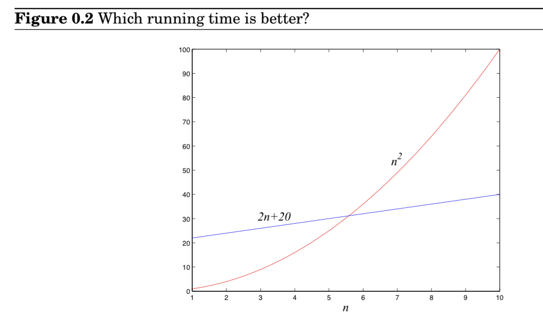
Sloppiness in the analysis of running times can lead to unacceptable level of inaccuracy in the result
Also possible to be too precise - the time taken by one such step depends crucially on the particular processor and details such as caching strategy.
Let and be functions from positive integers to positive reals. We say - f grows no faster than g - if there is a constant such that
Just as is an analog of , we can also define the analog of and as follows:
Reduction (DPV 7.1)
If any subroutine for task can also be used to solve , we say reduces to . Often, is solvable by a single call to ’s subroutine, which means any instance of can be transformed into an instance of such that can be deduced from
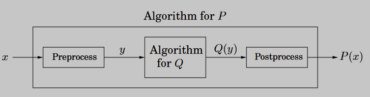
Reductions enhance the power of algorithms: Once we have an algorithm for problem Q (which could be shortest path, for example) we can use it to solve other problems.
Graphs
How is a graph represented?
Adjacency matrix
We represent a graph by an adjacency matrix, let there be vertices
For an undirected graph the matrix is symmetric since an edge can be taken in either direction
The presence of a particular edge can be cheked in constant time, but it takes space.
Adjacency List
With size proportional to the number of edges, consists of linked lists, one per vertex. The linked list for vertex holds the names of vertices to which has an outgoing edge.
Total size of the data structure is but checking for an edge is no longer constant time(requires sifting through ’s adjacency list)
Algorithms
Fibonacci(DPV 0)
Basic Arithmetic (DPV 1.1)
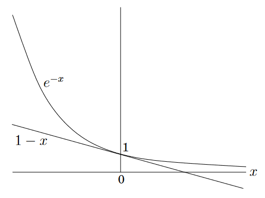
Incidentally, this function appears repatedly in our subject, in many guises. Here’s a sampling:
- is the power to which you need to raise in order to obtain .
- Going backward, it, , can also be seen as the number of times you must halve to get down to 1. This is useful when a number is halved at each iteration of an algorithm
- It, , is the number of bits in the binary representation of .
- It, , is also the depth of a complete binary tree with nodes
- It is even the sum , to within a constant factor.
Addition
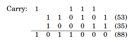
Basic property of numbers: The sum of any three single-digit numbers is at most two digits long (holds for any base b ≥ 2).
This simple rule gives us a way to add two numbers in any base: align their right-hand ends, and then perform a single right-to-left pass in which the sum is computed digit by digit, maintaining the overflow as a carry. Since we know each individual sum is a two-digit number, the carry is always a single digit, and so at any given step, three single-digit numbers are added.
We will not spell out the pseudocode because we are so familiar with it. We will go ahead and anlyze its efficiency: We want the answer expressed as a function of the size of the input: the number of bits of x and y, the number of keystrokes needed to type them in.
Suppose x and y are each n bits long; in this chapter we will consistently use the letter for the sizes of numbers. Then the sum of and is bits at most, and each individual bit of this sum gets computed in a fixed amount of time. The total running time for the addition algorithm is therefore of the form , where and are some constants; in other words, it is linear. Instead of worrying about the precise values of and , we will focus on the big picture and denote the running time as .
Some readers may be confused at this point: Why operations? Isn’t binary addition something that computers today perform by just one instruction? There are two answers.
First, it is certainly true that in a single instruction we can add integers whose size in bits is within the word length of today’s computers—32 perhaps. But, as will become apparent later in this chapter, it is often useful and necessary to handle numbers much larger than this, perhaps several thousand bits long. Adding and multiplying such large numbers on real computers is very much like performing the operations bit by bit. Second, when we want to understand algorithms, it makes sense to study even the basic algorithms that are encoded in the hardware of today’s computers. In doing so, we shall focus on the bit complexity of the algorithm, the number of elementary operations on individual bits—because this accounting reflects the amount of hardware, transistors and wires, necessary for implementing the algorithm.
Multiplication
algorithm for multiplying two numbers and is to create an array of intermediate sums, each representing the product of by a single digit of . These values are appropriately left-shifted and then added up. Suppose for instance that we want to multiply , or in binary notation, and .
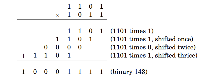
If and are both bits, then there are intermediate rows, with lengths of up to bits (taking the shifting into account). The total time taken to add up these rows, doing two numbers at a time, is:
But there are better ways to do this…
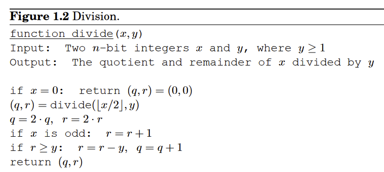
Division
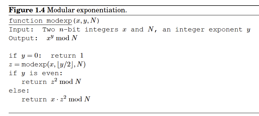
Modular Arithmetic (DPV 1.2, unfinished)
Just like multiplication, division works on computers with limited bits.
Modular arithmetic is a system for dealing with restricted ranges of integers. We define to be the remainder when is divided by ; that is, if with , then is equal to . This gives an enhanced notion of equivalence between numbers: and are congruent modulo if they differ by a multiple of , or in symbols
Another interpretation is that modular arithmetic deals with all the integers, but divides them into equivalence classes, each of the form for some between and
It uses n bits to represent numbers in the range and is usually described as follows:
- Positive integers, in the range , are stored in regular binary and have a
leading bit of 0.
- Negative integers , with , are stored by first constructing in binary, then flipping all the bits, and finally adding 1. The leading bit in this case is 1.
Here’s a much simpler way to think about it: any number in the range to is stored modulo . Negative numbers therefore end up as . Arithmetic operations like addition and subtraction can be performed directly in this format, ignoring any overflow bits that arise.
Hashing (DPV 1.5)
Hash Tables
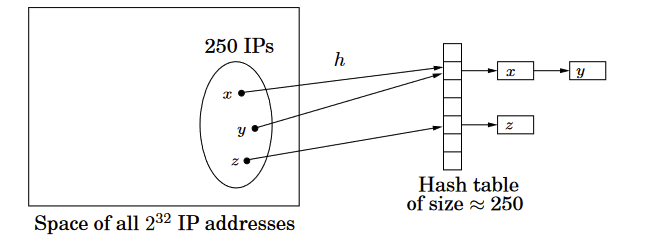
We will have an array of size and each key is hashed by hash function where . Each array element is a linked list
Hash Functions
- We want to make sure that hash collision is unlikely
- Otherwise we are wasting space
- We need randomization
- Pick a hash function randomly from some class of functions!
Let the number of buckets instead of , note that is a prime number
Let any IP address as a quadruple and we will fix any four numbers and map the address to .
We have defined the hash function
With this hash function,
Property: Consider any pair of distinct IP addresses , . If the coefficients are chosen uniformly at random from , then
This condition guarantees that the expected lookup time for any item is small.
Proof:
Since and are distinct, these quadruples must differ in some component; without loss of generality let us assume that . We wish to compute the probability
that is, the probability that
This last equation can be rewritten as
Suppose that we draw a random hash function ha by picking at random. We start by drawing , , and , and then we pause and think:
What is the probability that the last drawn number is such that equation above holds?
We know
- So far the LHS evaluates to
- Since is prime and , has a unique inverse mod
Thus for previous equation to hold,
The probability of this happening is
Universal Hash Functions
Family of hash functions that satisfy the following property:
For any two distinct data items and , exactly of all the hash functions in map and to the same bucket, where is the number of buckets
In our example, we used the family
Which is an group of universal hash functions
In other words, for any two data items, the probability these items collide is 1/n if the hash function is randomly drawn from a universal family.
Divide and Conquer (DPV 2)
Recurrence Relationships (DPV 2.2)
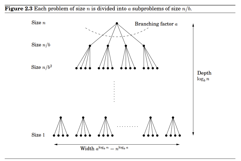
Divide and conquer often follow a generic pattern of runtime:
To prove master theorem,
we will assume that n is a power of b (this will not influence the final bound because n is at most a multiplicative factor of b away from some power of b)
Notice that the size of the subproblems decrease by a factor of b with each level of recursion, and therefore reaches the base case after levels. Its branching factor is , so the k-th level of the tree is made up of subproblems, each of size . The total work done at this level is
As goes from 0 to , these numbers form a geometric series with ratio . Therefore we can find the sum by three cases:
-
- The series is decreasing, and its sum is just given by the first term
-
- We will have counts of the first term
-
-
- The series is increasing, and its sum is given by its last term
-
-
Multiplication (DPV 2.1)
Gauss’s trick:
Product of two complex numbers:
Can in fact be done with just three terms because:
Using the same idea, if and are two n-bit integers, we can represent them as left and right halves of bits
We have recursion expression of
for this multiplication relationship
But we can use Guss’s trick, we only need to compute the multiplication since
(Karatsuba Algorithm)
MergeSort
“Split the list into two halves, recursively sort each half, and merge the two sorted sublists”
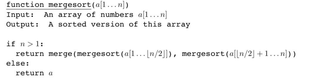
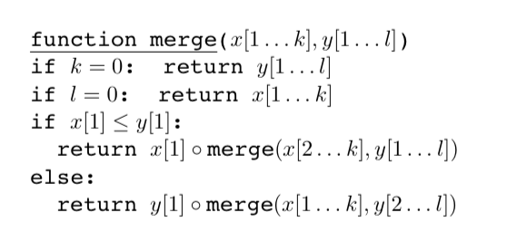
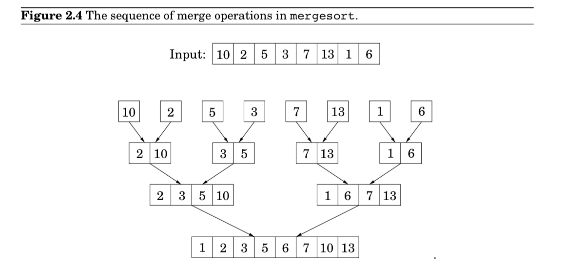
The merge procedure does a constant amount of work per recursive call, thus and the overall time taken by mergesort:
We will also define an iterative version of mergesort, where means to append an element to the end of an array and means to remove an element at the front of the array and return it.
Reason of why sorting using comparison must be at least is because every permutation of the elements must be present in the leaves of the sorting algorithm and therefore the complexity of the tree representing the sorting algorithm must have
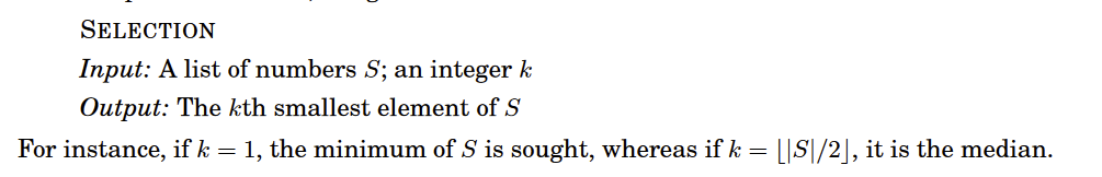
Median
When looking for a recursive solution, it is paradoxically often easier to work with a more general version of the problem—for the simple reason that this gives a more powerful step to recurse upon. In our case, the generalization we will consider is selection
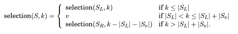
Divide and Conquer for selection:
For any number , imagine splitting list into three categories: elements smaller than , those equal to (there might be duplicates), and those greater than .
For instance, if the array :

is put to split on , then

We can check is in which sub-array by using length of each array
Worst case:
- We select to be the smallest/largest element of the array each time, causing array to only shrink by 1.
We will define a good selection of to at least strip away 25% of the original array.
Therefore
Matrix Multiplication (DPV 2.5)
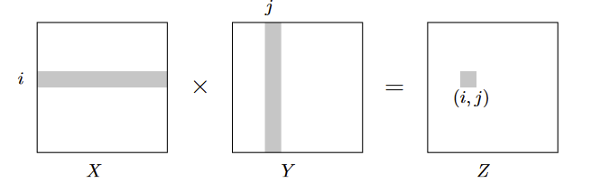
Matrix Multiplication can be viewed as blocks
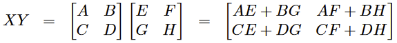
But it is still , by:
Turns out can be computed from just seven subproblems
where
The new runtime is
Fast Fourier Transform (DPV 2.6)

Product of two degree-d polynomials is a polynomial of degree 2d:
Then
and will have coefficients
Where
Computing each takes and results to an overall steps since we have coefficients
So therefore do we have a faster algorithm for solving this problem?
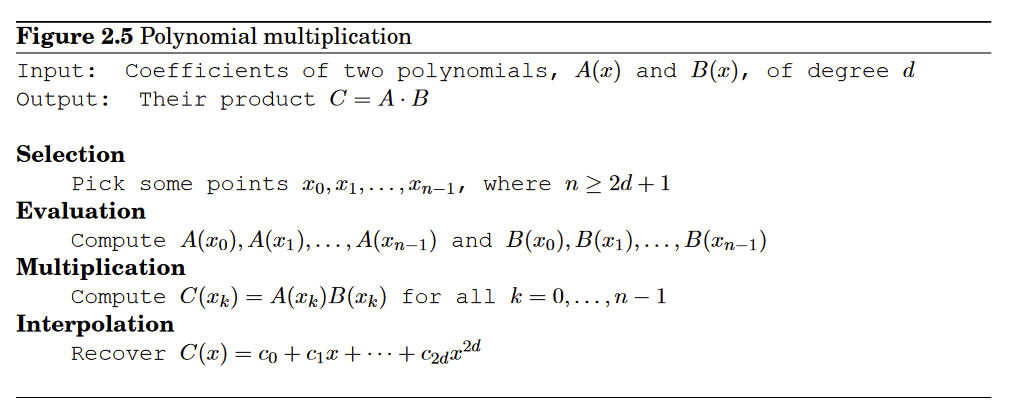
Here are coefficients of the functions (describing the function), and are point to be evaluated at the function.
So now we have evaluted the polynomial at those representation points, we have multiplied the values to obtain values, how do we interpolate back?
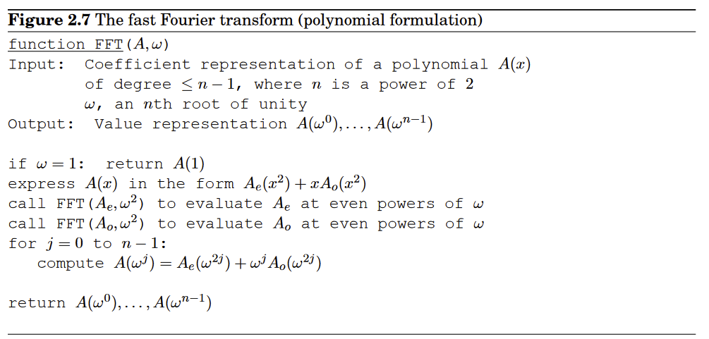
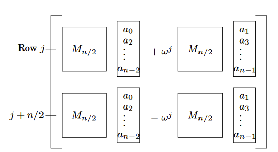
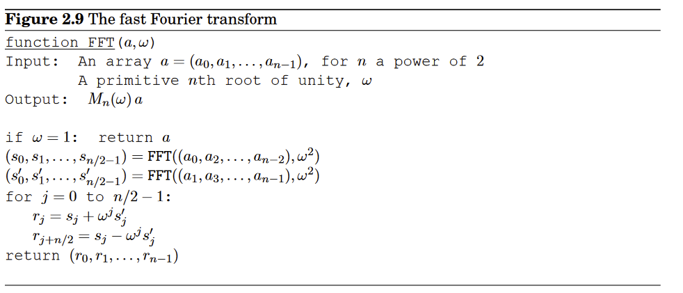
The definitive FFT Algorithm:
The FFT takes as input a vector and a complex number whose powers are complex n-th roots of unity.
We can apply divide and conquer to the matrix multiplication steps
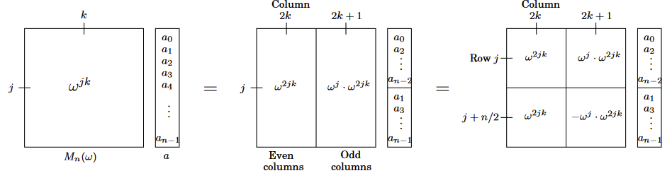
The final product is the vector
Summary:
The divide-and-conquer step of the FFT can be drawn as a very simple circuit. Here is how a problem of size is reduced to two subproblems of size (for clarity, one pair of outputs is singled out):
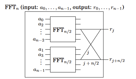
the edges are wires carrying complex numbers from left to right. A weight of means “multiply the number on this wire by .
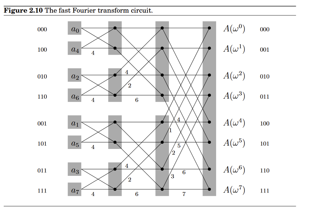
- For inputs there are levels, each with nodes, for a total of operations
- the inputs are arranged by increasing last bit of the binary representation of their index, resolving ties by looking at the next more significant bit(s).
- For , The resulting order in binary, 000, 100, 010, 110, 001, 101, 011, 111
- There is a unique path between each input and each output
- This path is most easily described using the binary representations of j and k (shown in Figure 10.4 for convenience). There are two edges out of each node, one going up (the 0-edge) and one going down (the 1-edge).
- To get to A(ωk) from any input node, simply follow the edges specified in the bit representation of k, starting from the rightmost bit
- On the path between and ), the labels add up to .
- Contribution of input to output is
- Notice that the FFT circuit is a natural for parallel computation and direct implementation in hardware.
Graphs (DPV 3 + 4)
DFS (Depth-first Search) in undirected graphs (DPV 3.2)
Surprisingly versatile linear-time procedure that reveals a wealth of information about a graph
Explore
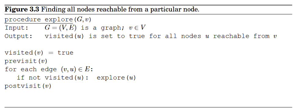
Depth-First Search Algorithm (DFS)
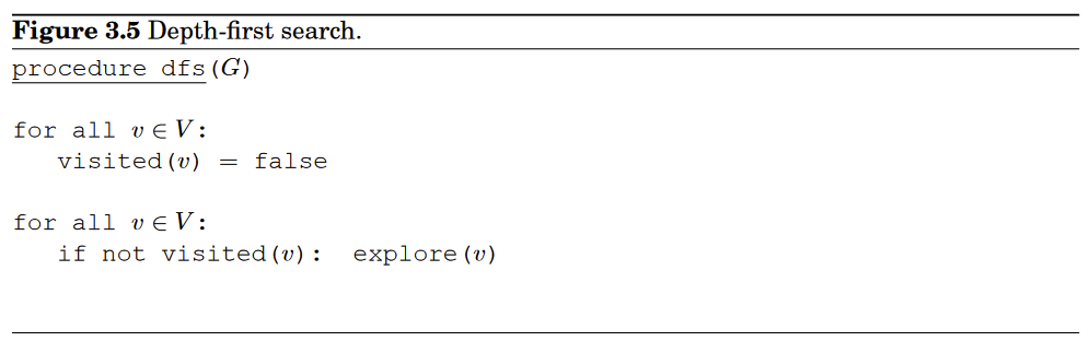
First step:
Marking visited to false,
Second step:
Every edge examined exactly twice (for an edge , we visit from and ) ⇒
Connected Components
We can also check what connected components exist in the graph by simply modifying a bit in the DFS algorithm

Where here identifies the connect component to which belongs
is initialized to zero and incremented each time calls
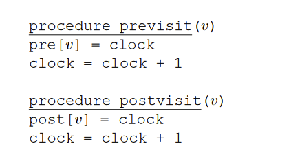
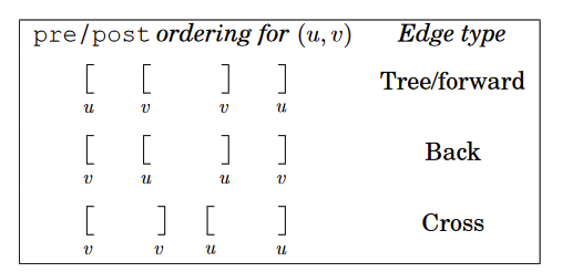
Previsit and postvisit ordering
We will also note down the times of two important events, the moemnt of first discovery and of final departure.
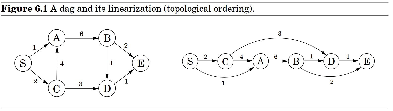
Directed Acyclic graphs (DAGs) (DPV 3.3.2)
Good for modeling relationships like causalities, hierarchies, and temporal dependencies.
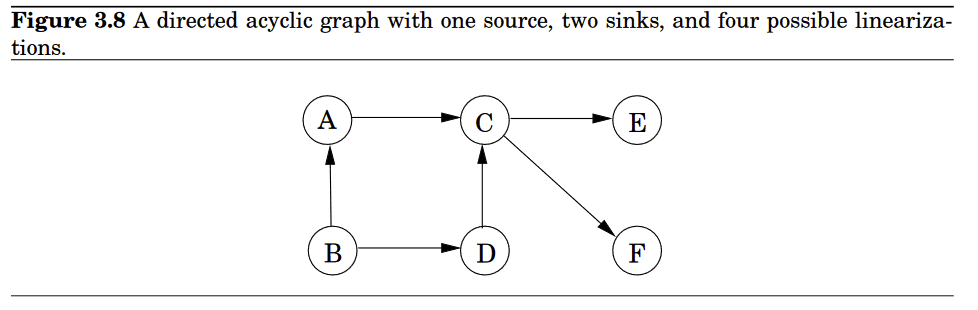
All DAGs can be linearized. ⇒ perform tasks in decreasing order of their post numbers
only edges in a graph for which are back edges ⇒ and dag cannot have back edges ⇒ In a DAG, every edge leads to a vertex with a lower number
So therefore
Also, since every DAG has at least one source and one sink…We can do this linearization
- Find a source, output it, and delete it from graph
- Repeat until the graph is empty
Strongly Connected Components
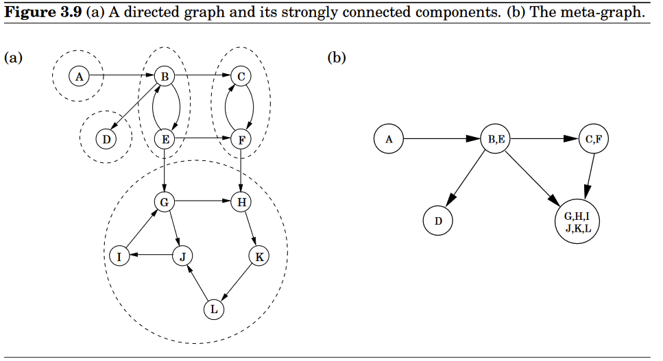
Two nodes and of a directed graph are connected if there is a path from to and a path from to .
And… turns out the meta-graph can be found in linear time by making further use of DFS.
Property 1: If the subroutine is started at node , then it will terminate precisely when all nodes reachable from have been visited.
So if we call on a node that lies somewhere in a strongly connected component, then we will retrieve exactly that component.
Property 2: The node that receives the highest number in a DFS must lie in a source strongly connected component.
Property 3: If and are strongly connected components, and there is an edge from a node in to a node in , then the highest number in is bigger than the highest number in .
Proof of property 3:
In proving Property 3, there are two cases to consider. If the depth-first search visits component before component , then clearly all of and will be traversed before the procedure gets stuck (see Property 1). Therefore the first node visited in will have a higher post number than any node of . On the other hand, if gets visited first, then the depth-first search will get stuck after seeing all of but before seeing any of C, in which case the property follows immediately.
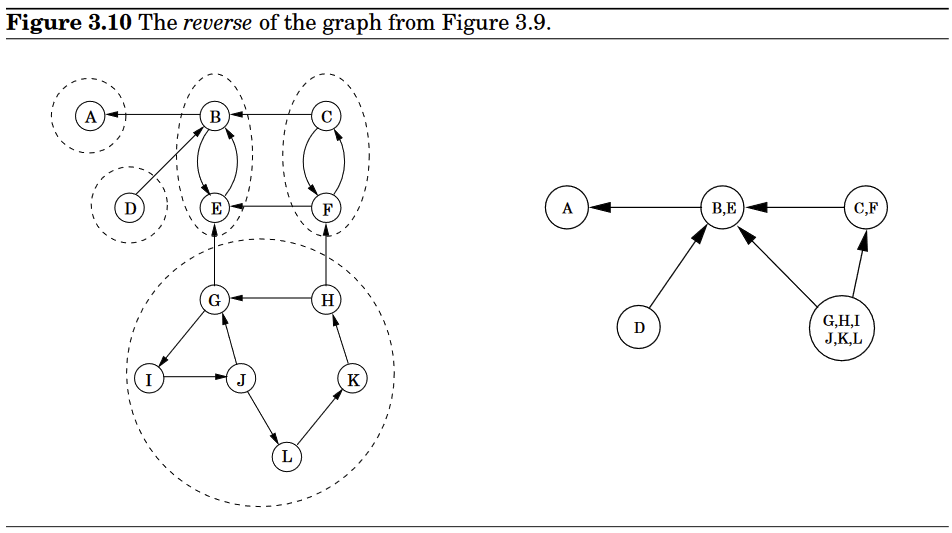
We can use the reverse graph and property 2 to find a node from the component of graph
Once we have found the first strongly connected component and deleted it from the graph, the node with the highest post number among those remaining will belong to a sink strongly connected component of whatever remains of . Therefore we can keep using the post numbering from our initial depth-first search on to successively output the second strongly connected component, the third strongly connected component, and so on. The resulting algorithm is this.
- Run DFS on
- Run the undirected connected components algorithm on , and during the DFS, process the vertices in decreasing order of their numbers from step 1.
This is linear time, only the constant is about twice of normal DFS search
Paths in Graphs: Distances (DPV 4.1)
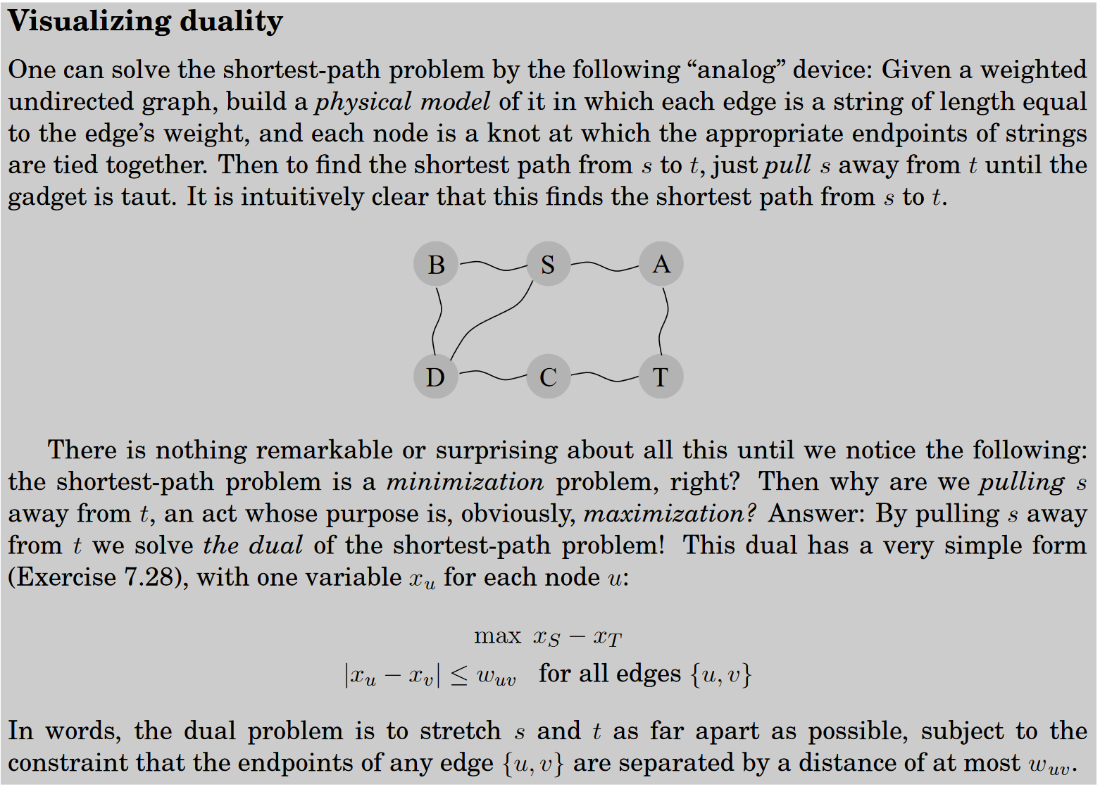
The distance between two nodes is the length of the shortest path between them.
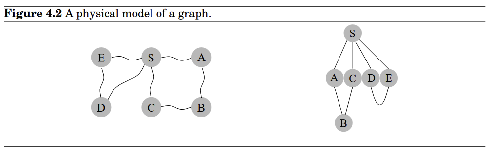
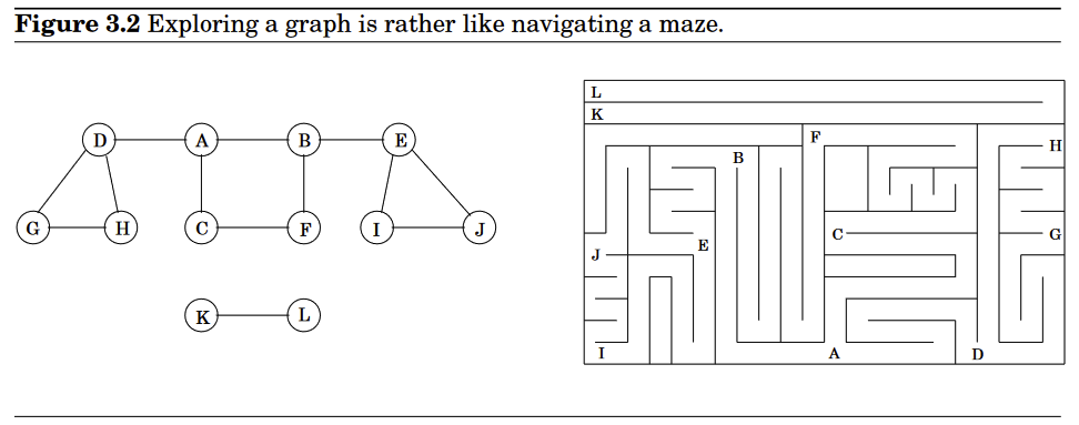
To get a concrete feel for this notion, consider a physical realization of a graph that has a ball for each vertex and a piece of string for each edge. If you lift the ball for vertex s high enough, the other balls that get pulled up along with it are precisely the vertices reachable from s. And to find their distances from s, you need only measure how far below s they hang.
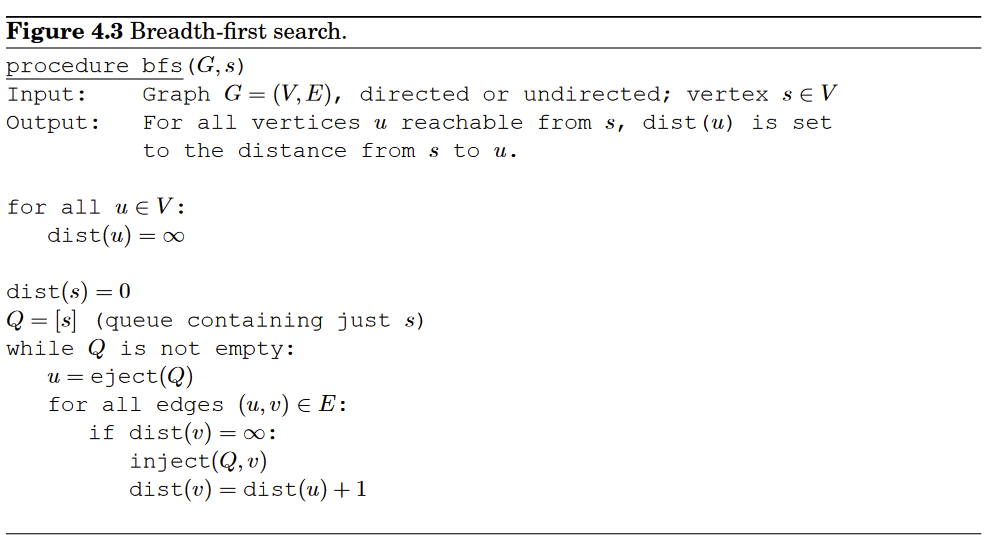
Breadth-First Search (BFS) (DPV 4.2)
Initially the queue consists only of the root, , the one node at distance . And for each subsequent distance , there is a point in time at which contains all the nodes at distance and nothing else. As these nodes are processed (ejected off the front of the queue), their as-yet-unseen neighbors are injected into the end of the queue.
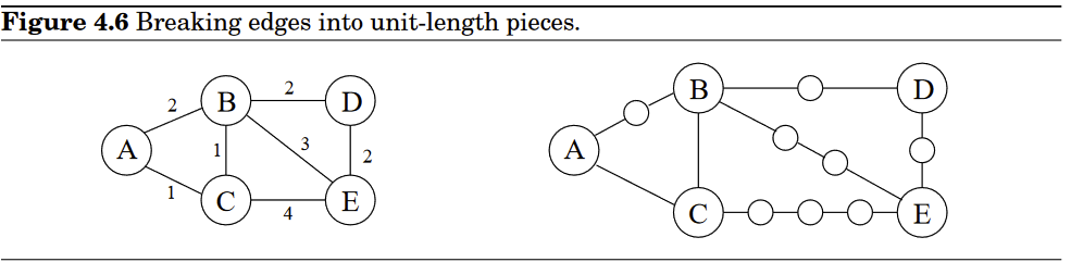
Lengths on Edges (DPV 4.3)
We will annotate every edge with .
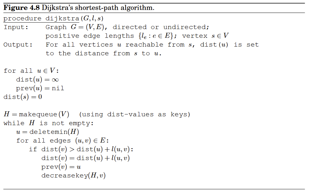
Dijkstra’s Algorithm (DPV 4.4)
we can think of Dijkstra’s algorithm as just BFS, except it uses a priority queue instead of a regular queue, so as to prioritize nodes in a way that takes edge lengths into account.
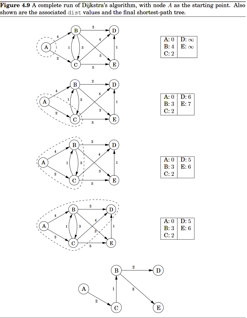
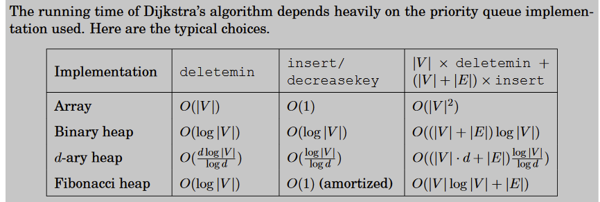
Runtime Analysis:
Dijkstra’s algorithm is structurally identical to breadth-first search. However, it is slower because the priority queue primitives are computationally more demanding than the constant-time ’s and ’s of BFS. Since makequeue takes at most as long as insert operations, we get a total of and / operations. The time needed for these varies by implementation; for instance, a binary heap gives an overall running time of .
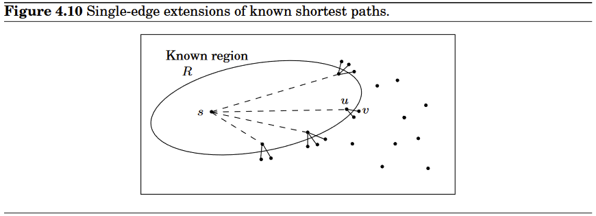
Priority Queue Implemention in Dijkstra (DPV 4.5)
Array
The simplest implementation of a priority queue is as an unordered array of key values for all potential elements (the vertices of the graph, in the case of Dijkstra’s algorithm).
Initially, these values are set to . An insert or decreasekey is fast, because it just involves adjusting a key value, an operation. To , on the other hand, requires a linear-time scan of the list.
Binary Heap
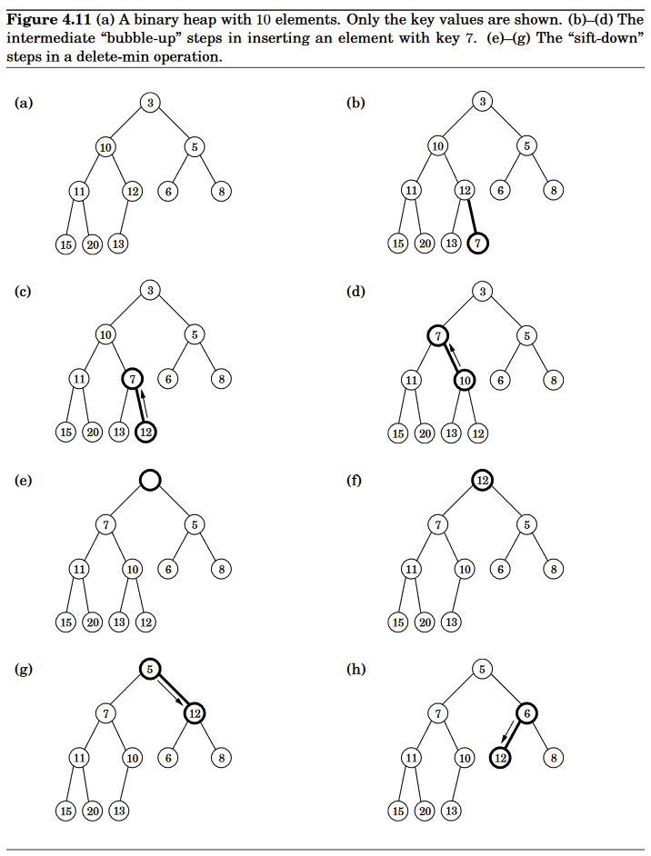
Elements are stored in a complete binary tree, in which each level is filled in from left to right, and must be full before the next level is started.
And special ordering constraint: the key value of any node of the tree is less than or equal to that of its children.
To , place the new element at the bottom of the tree (in the first available position), and let it “bubble up.” That is, if it is smaller than its parent, swap the two and repeat (Figure 4.11(b)–(d)). The number of swaps is at most the height of the tree, which is when there are elements.
A is similar, except that the element is already in the tree, so we let it bubble up from its current position.
To , return the root value. To then remove this element from the heap, take the last node in the tree (in the rightmost position in the bottom row) and place it at the root. Let it “sift down”: if it is bigger than either child, swap it with the smaller child and repeat (Figure 4.11(e)–(g)). Again this takes O(log n) time.
The regularity of a complete binary tree makes it easy to represent using an array. The tree nodes have a natural ordering: row by row, starting at the root and moving left to right within each row. If there are n nodes, this ordering specifies their positions within the array. Moving up and down the tree is easily simulated on the array, using the fact that node number has parent and children and
d-ary Heap
A d-ary heap is identical to a binary heap, except that nodes have d children instead of just two. This reduces the height of a tree with elements to .
Inserts are therefore speeded up by a factor of . operations, however, take a little longer, namely
Negative-value edges? (DPV 4.6.1)
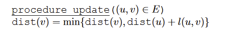
Dijkstra’s method can be thought as a sequence of “Update” operations
But Dijkstra’s method will mark off vertices that have been used to calculate shorter distances, this usually cannot be the case with negative-value edges because now updated vertices might receive an update from a negative edge.
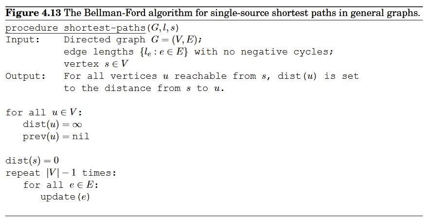
Detecting Negative Cycles (DPV 4.6.2)
In such situations, it doesn’t make sense to even ask about shortest paths. There is a path of length 2 from A to E. But going round the cycle, there’s also a path of length 1, and going round multiple times, we find paths of lengths 0, −1, −2, and so on.
Fortunately, it is easy to automatically detect negative cycles and issue a warning. Such a cycle would allow us to endlessly apply rounds of update operations, reducing dist estimates every time.
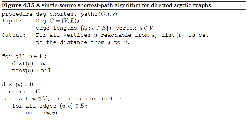
Shortest Paths in DAGs that doesn’t have negative cycles (DPV 4.7)
There are two subclasses of graphs that automatically exclude the possibility of negative cycles:
- graphs without negative edges
- Dijkstra
- graphs without cycles
- Can be solved in linear time!
Linearize (that is, topologically sort) the dag by depth-first search, and then visit the vertices in sorted order, updating the edges out of each.
Greedy Algorithms (DPV 5)
A player who is focused entirely on immediate advantage is easy to defeat. But in many other games such as Scrabble, it is possible to do quite well by simply making whichever move seems best at the moment
Minimum Spanning Trees
Suppose you are asked to network a collection of computers by linking selected pairs of them. Each link also has a maintenance cost, reflected in that edge’s weight. What is the cheapest possible network?
Trees
A tree is an undirected graph that is connected and acyclic
Property:
- A tree on nodes has edges
- Any connected, undirected graph with is a tree
- An undirected graph is a tree if and only if there is a unique path between any pair of nodes
The cut property:
Suppose edges are part of a minimum spanning tree of . Pick any subset of nodes for which does not cross between and , and let be the lightest edge across this partition. Then is part of some MST.
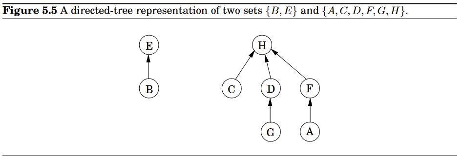
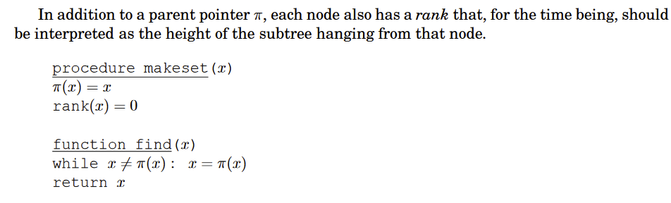
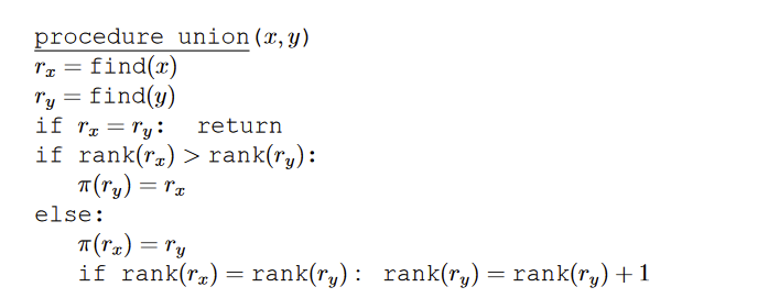
Data structure for disjoint sets - Union by rank
Faster find:
When we want to merge sets, if the representatives (roots) of the sets are and , do we make point to or the other way around? Since tree height is the main impediment to computational efficiency, a good strategy is to make the root of the shorter tree point to the root of the taller tree.
Properties:
-
- Any node of rank k has at least nodes in its tree
- If there are elements overall, there can be at most nodes of rank
Kruskal’s Method
Sort the edges by their weights, everytime check if the smallest edge would add a cycle to the graph. If it doesn't then it gets added to the graph.
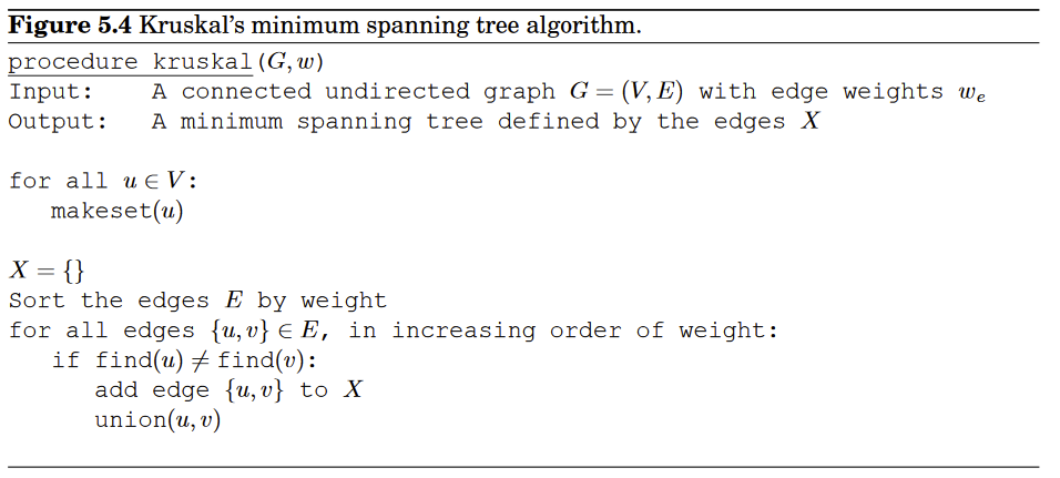
for sorting edges and for unino and find operations
But if the weights are small so that sorting can be done in linear time? Can we perform and faster than ?
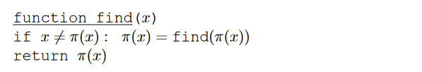
during each , when a series of parent pointers is followed up to the root of a tree, we will change all these pointers so that they point directly to the root ⇒ use the faster
Now the amortized cost of and is
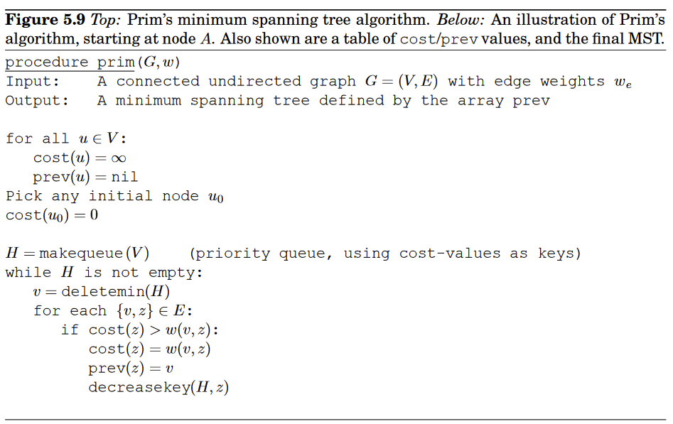
Prim’s Method
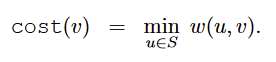
Start from an arbitraty node, at each step we added the shortest edge connecting some node already in the tree to one that isn't yet.
So obtain a subgroup and another subgroup that contains vertices not selected in the first subgroup. Whatever edges that hasn't been selected yet that connects the first group with the second and has the smallest weight will be selected.
Huffman Encoding
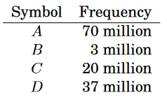
What is the most economic way of writing strings consisting of letters A,B,C,D?
The obvious choice is to use bits per symbol—say codeword for , for , for , and for - in which case megabits are needed in total. Can there possibly be a better encoding than this?
In search of inspiration, we take a closer look at our particular sequence and find that the four symbols are not equally abundant.
Is there some sort of variable-length encoding, in which just one bit is used for the frequently occurring symbol A, possibly at the expense of needing three or more bits for less common symbols?
A danger with having codewords of different lengths is that the resulting encoding may not be uniquely decipherable. For instance, if the codewords are , the decoding of strings like is ambiguous. We will avoid this problem by insisting on the prefix-free property: no codeword can be a prefix of another codeword.
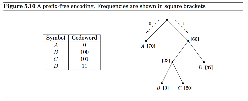
To measure how “good” a coding tree is, we want a tree whose leaves each correspond to a symbol and minimizes the overall length of the encoding
Tells us that the two symbols with the smallest frequencies MUST be at the bottom of the optimal tree, as children of lowest internal node. ⇒ because otherwise swapping whatever node with either of those two would increase performance.
This suggests that we start constructing the tree greedily: find the two symbols with the smallest frequencies, say and , and make them children of a new node, which then has frequency
There is another way to write this cost function that is very helpful. Although we are only given frequencies for the leaves, we can define the frequency of any internal node to be the sum of the frequencies of its descendant leaves; this is, after all, the number of times the internal node is visited during encoding or decoding. During the encoding process, each time we move down the tree, one bit gets output for every nonroot node through which we pass.
And therefore
The cost of a tree is the sum of the frequencies of all leaaves and internal nodes, except the root
Entropy
Average number of bits needed to encode a single draw from the distribution
Measures the randomness of a set of mixed elements
Horn Formula
A framework for doing computer doing logical reasoning!
A literal is either: a variable or a variable’s negation
Then we have two kinds of caluses:
- Implications, left hand side is and AND of any number of positive literals and right hand is a single positive iteral
- Pure negative clauses, consisting of an OR of any number of negative literals
Given a set of clauses, the goal is to do satisfying assignment - determine whether there is a consistent explanation: an assignment of values to the variables that satisfies all the clauses.
Our approach:
- Start with all variables
- and proceed to set some of them to
- one by one and only if we absolutely have to because an implication would be violated
Horn formulas lie at the heart of Prolog (“programming by logic”), a language in which you program by specifying desired properties of the output, using simple logical expressions
To see why the algorithm is correct, notice that if it returns an assignment, this assignment satisfies both the implications and the negative clauses, and so it is indeed a satisfying truth assignment of the input Horn formula. So we only have to convince ourselves that if the algorithm finds no satisfying assignment, then there really is none. This is so because our “stingy” rule maintains the following invariant:
If a certain set of variables is set to true, then they must be true in any satisfying assignment.
Set cover
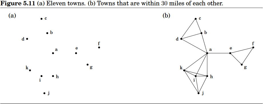
County is in its early stages of planning and is deciding where to put schools. There are only two constraints: each school should be in a town, and no one should have to travel more than 30 miles to reach one of them.
What is the minimum number of schools needed?
Let be the set of towns within 30 miles of town , a school at will esentially “cover”these other towns. Then how many sets must be picked in order to cover all the towns in the country?
Greedy solution:
- Repeat until all elements of are covered
- Pick the set with the largest number of uncovered elements
But we will see that this is not optimal, but it’s not too far off, so let’s modify this.
Suppose contains elements and that the optimal cover consists of sets, then the greedy algorithm will use at most sets.
Let be the number of elements still not covered after iterations of the greedy algorithm, since these remaining elements are covered by the optimal sets
there must be some set with at least of them.
Therefore, the greedy strategy will ensure that
Which implies .
If we use an inequality
Therefore
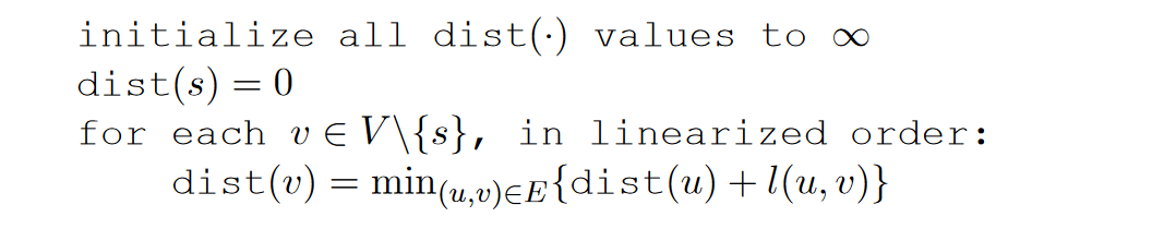
Dynamic Programming (DPV 6)
Shortest Paths in DAGS
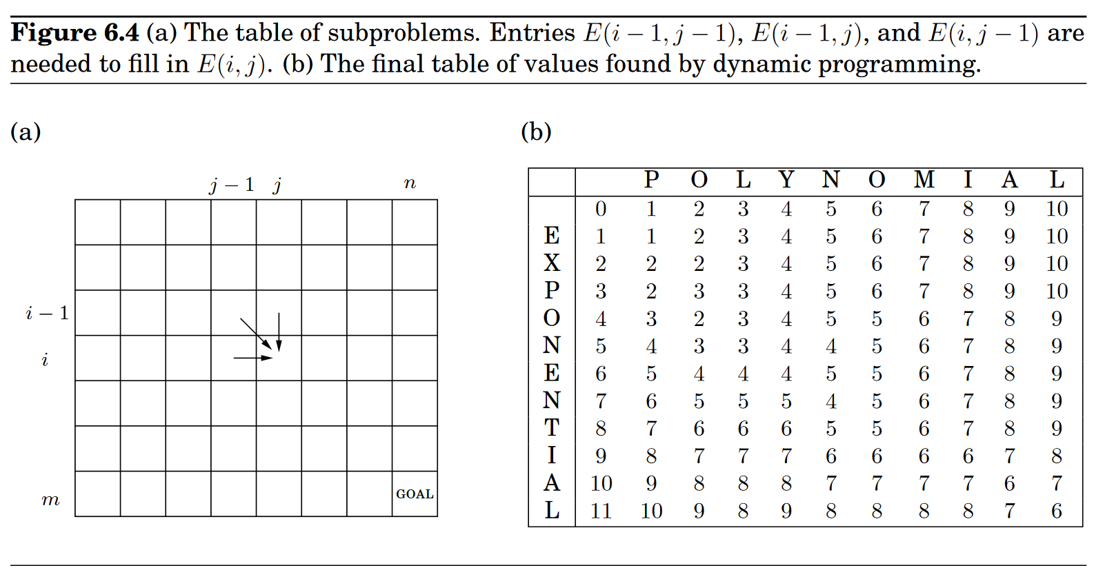
In this particular graph, we see that in order for us to find shortest distance from to
We can compute all distances in a single pass:
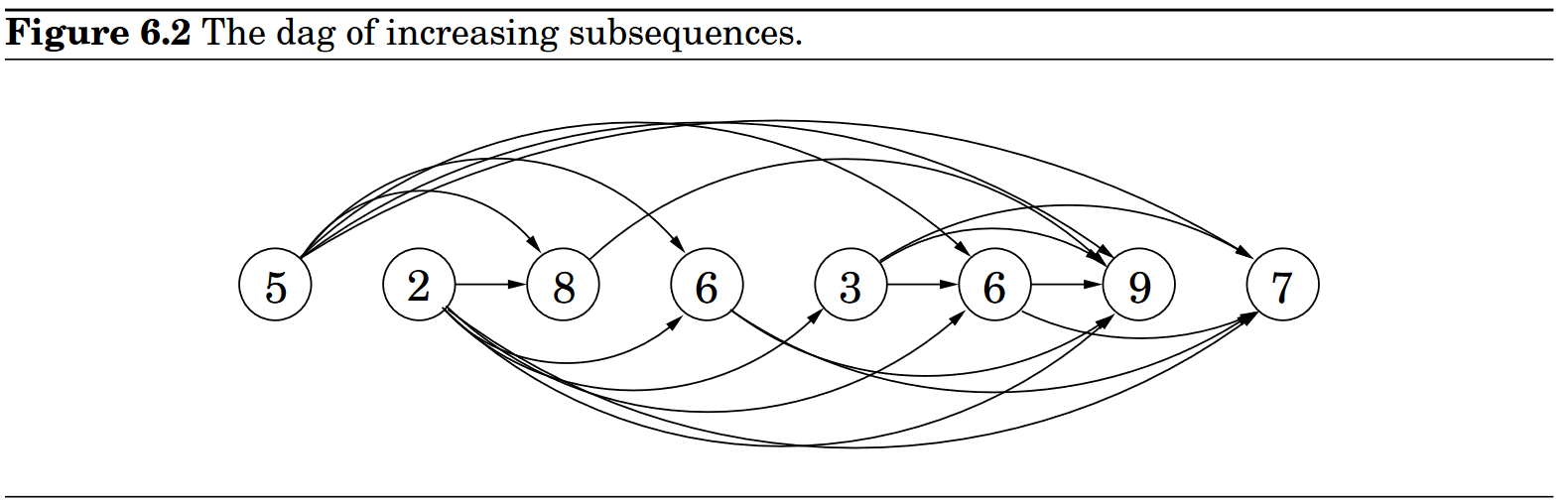
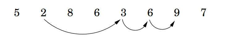
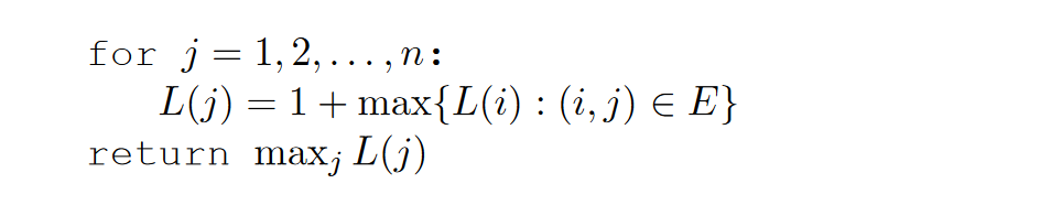
Longest Increasing Subsequences
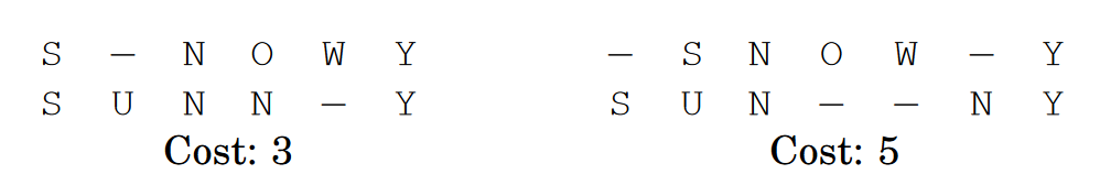
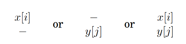
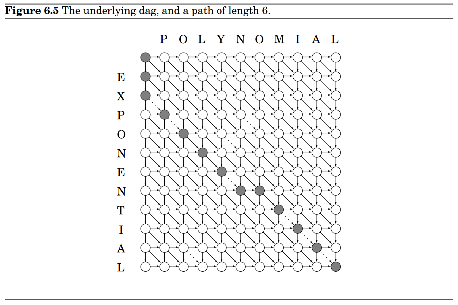
String Edit Distance
Knapsack
During a robbery, a burglar finds much more loot than he had expected and has to decide what to take. His bag (or “knapsack”) will hold a total weight of at most pounds. There are items to pick from, of weight and dollar value . What’s the most valuable combination of items he can fit into his bag?
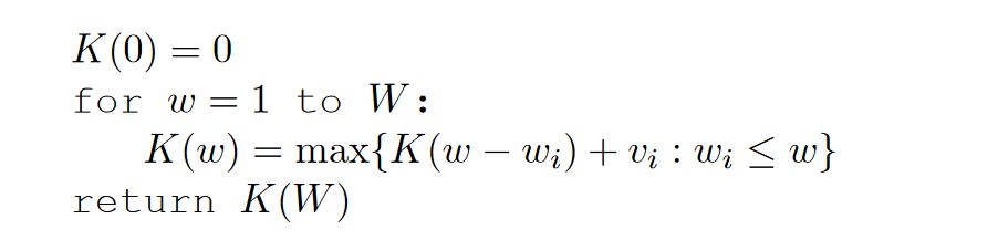
Knapsack with repetition
If there are unlimited quantities of each item available
If the optimal solution to includes item i, then removing this item from the knapsack leaves an optimal solution to .
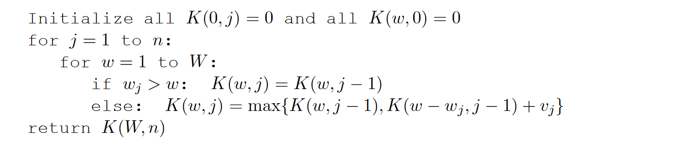
Kanpsack without repetition
(Chain) Matrix Multiplication
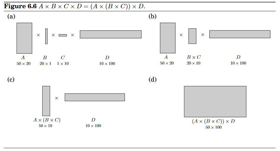
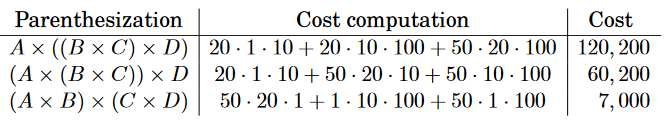
Observation: Order of multiplications make a big difference in the final runtime!
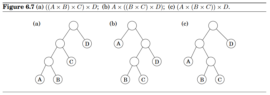
For a tree to be optimal, its subtrees must also be optimal.
Let the subproblems corresponding to the subtrees be in the form . For , we define a function
When there’s nothing to multiply ⇒
We can split the subproblem into smaller subproblems
The subproblems constitute a two-dimensional table, each of whose entries take time to compute, the overall runtime is thus .
Shortest Paths
We started this chapter with a dynamic programming algorithm for the elementary task of finding the shortest path in a dag. We now turn to more sophisticated shortest-path problems and see how these too can be accommodated by our powerful algorithmic technique.
Shortest Reliable Paths
In a communications network, for example, even if edge lengths faithfully reflect transmission delays, there may be other considerations involved in choosinga path. For instance, each extra edge in the path might be an extra “hop” fraught with uncertainties and dangers of packet loss.
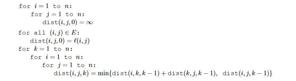
All-pairs shortest paths (Flyd-Warshall Algorithm)
What if we want to find the shortest path not just between s and t but between all pairs of vertices? One approach would be to execute our general shortest-path algorithm from Bellman-Ford (since there may be negative edges) times, once for each starting node. The total running time would then be . We’ll now see a better alternative, the dynamic programming-based Floyd-Warshall algorithm.
If we number the vertices as , and denote as the length of the shortest path from to in which only nodes can be used as intermediates.
What happens when we expand the intermediate set to include an extra node k? We must reexamine all pairs i, j and check whether using k as an intermediate point gives us a shorter path from i to j.
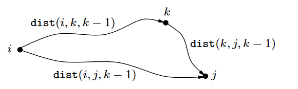
Then using gives us a shorter path from to iff
So the algorithm(Floyd-Warshall Algorithm )
Traveling Salesman Problem (TSP)
A traveling salesman is getting ready for a big sales tour. Starting at his hometown, he will conduct a journey in which each of his target cities is visited exactly once before he returns home. Given the pairwise distances between cities, what is the best order in which to visit them, so as to minimize the overall distance traveled?
If we denote the cities by , the salesman’s hometown being 1, and let be the matrix of intercity distances, the goal is to design a tour that starts and ends at 1, including all other cities exactly once, and has minimum total length.
Bruteforce takes time, and although DP improves this runtime a lot it is still not possible to solve this in polynomial time.
Subproblems:
For a subset of cities that includes 1, and , let be the length of the shortest path visiting each node in exactly once, starting at 1 and ending at .
When , wedefine since the path cannot both start and end at 1.
The subproblems are ordered by , the whole algorithm is:
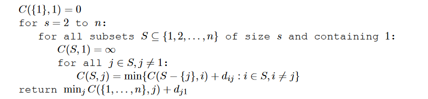
There are at most subproblems, and each one takes linear time to solve, so the overall complexity is
Independent Sets in Trees
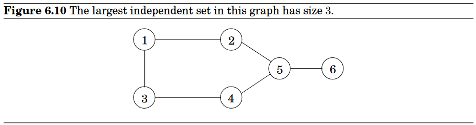
A subset of nodes is an independent set of graph if there are no edges between them.
Like before, we can form this problem into a tree of nodes representing sub-problems
We will define the subproblem( is a node in the tree, which also represents a node in graph):
We will simply select any node in graph vertices as the root of the tree
Our goal is to find ⇒ represents the root of the tree
If the independent set includes , then we get one point for it, but we aren’t allowed to include the children of (since they are directly connected to )—therefore we move on to the grandchildren.
The number of subproblems is exactly the number of vertices and with a little care the runtime can be made linear
Linear Programming and Reductions (DPV 7)
Linear Programming (DPV 7.1 + 7.4)
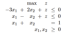
We are given a set of variables, and we want to assign real values to them so as to
- satisfy a set of linear equations / inequalities involving these variables
- maximize or minimize a given linear objective function
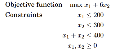
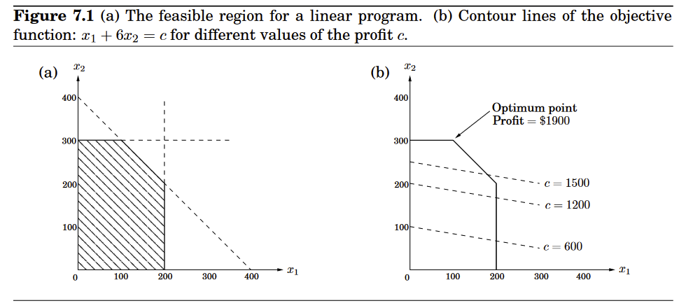
An inequality designates a half-space, the region on one side of the line.
Thus the set of all feasible solutions of this linear program, that is, the points (x1, x2) which satisfy all constraints, is the intersection of five half-spaces, and is a convex polygon.
We want to find the point in this polygon at which the objective function—the profit—is maximized. The points with a profit of c dollars lie on the line , which has a slope of .
Since the goal is to maximize c, we must move the line as far up as possible, while still touching the feasible region. The optimum solution will be the very last feasible point that the profit line sees and must therefore be a vertex (or edge) of the polygon, as shown in the figure.
Standard Form of LP (DPV 7.1)
- All variables are nonnegative
- Constraints are all equations
- objective function is to be minimized
Duality of LP (DPV 7.4)
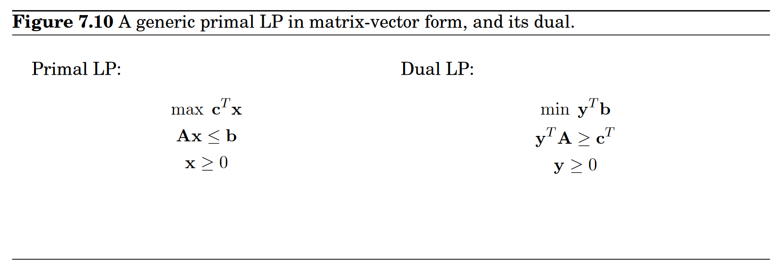
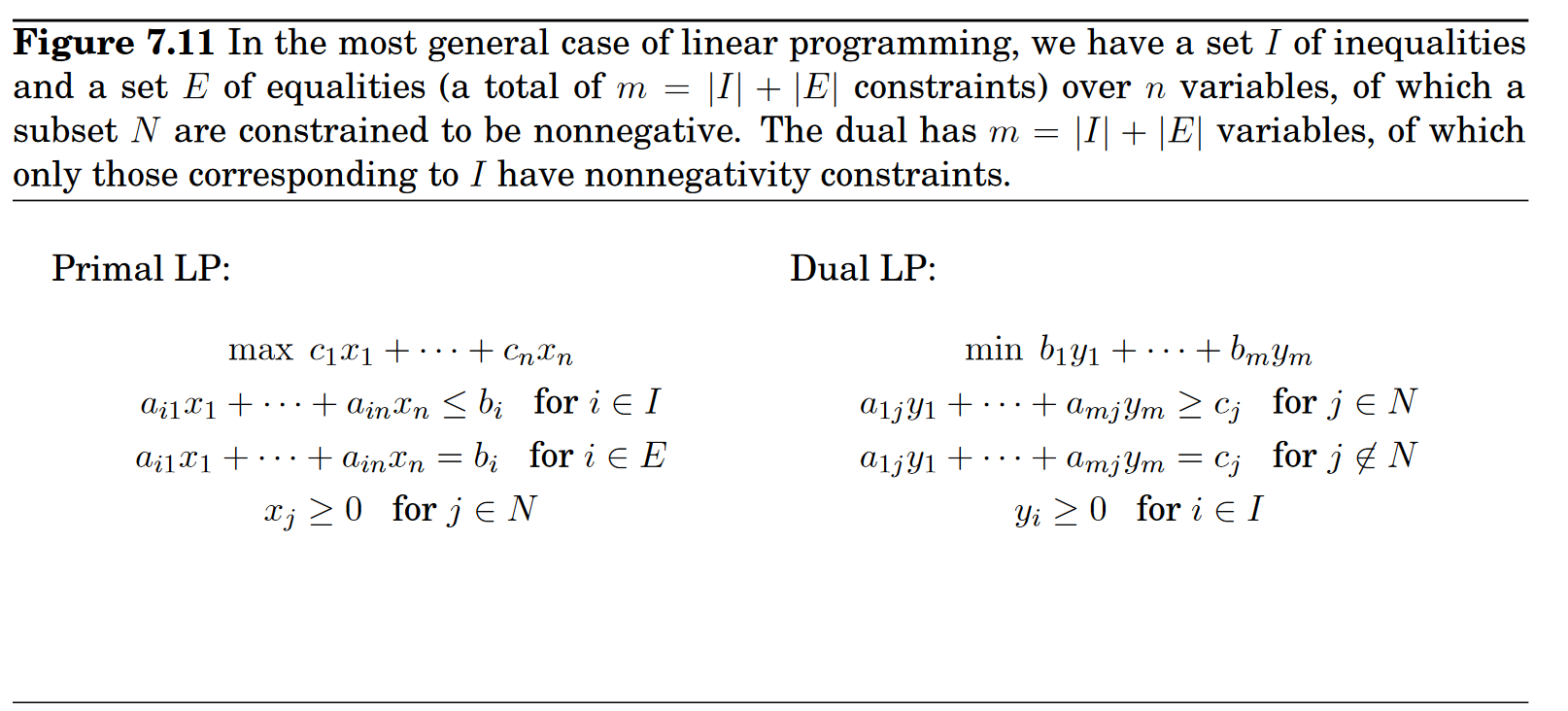
Duality theorem: If a linear program has a bounded optimum, then so does its dual, and the two optimum values coincide
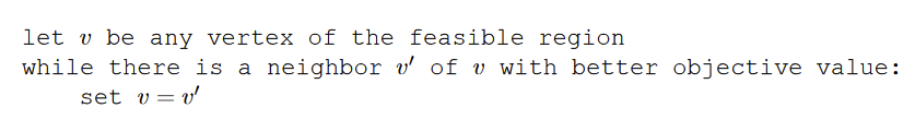
Simplex Algorithm
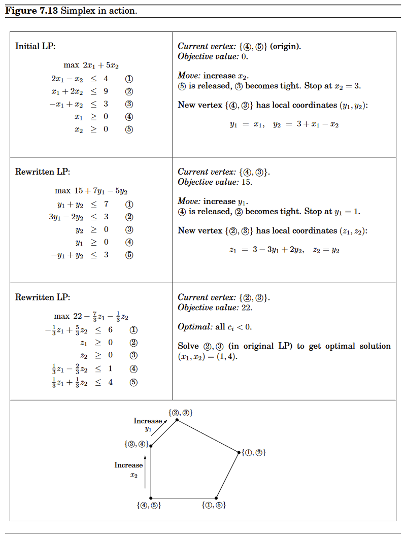
Fact: each vertex is the unique point at which some subset of hyperplanes meet.
So to find a vertex:
- Pick a subset of the inequalities. If there is a unique point that satisfies them with equality, and this point happens to be feasible, then it is a vertex.
- Each vertex (of dimension n) is specified by a set of n inequalities.
- Note that there might be vertices that are degenrate
- They could be found by different subsets of inequalities
- We just pretend they don’t exist for now
- Two vertices are neighbors if they have defining inequalities in common.
Suppose we have a generic LP
For each iteration, we want to
- Check if the current vertex is optimal
- Determine where to move next
Note:
The origin is a vertex that we can start with.
- The current vertex(origin) is optimal iff
- We can increase some for which (release the tight constraint ⇒ until we hit some other constraint (loose ⇒ tight)
Now we arrived at some other vertex
Then we transform into the origin(shifting the coordinate system from the usual to the “local” view of )
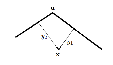
These local coordinates consist of (appropriately scaled) distances to the hyperplanes (inequalities) that define and enclose :
- ⇒
The revised “local” LP has the following three properties:
- It includes the inequalities , which are simply the transformed versions of the inequalities defining
- is the origin in y-space
- Cost function becomes where is the value of the objective function at and is a transformed cost vector
The simplex function moves from vertex to neighboring vertex, stopping when the objective function is locally optimal, that is, when the coordinates of the local cost vector are all zero or negative.
Runtime Analysis
Suppose there are variables and inequalities
At each iteration:
- Each neighbors share inequalities with the current vertex, at most neighbors
- Choose which inequality to drop () and which new one to add ()
- Naive way to perform each iteration
- Check each potential neighbor to see whether it really is a vertex of the polyhedron and to determine its cost
- Finding cost is just a dot product
- Checkingif it is a true vertex involves a solving a system of linear equations with equations in unknowns
- by Gaussian Elimination
- per iterations
- Check each potential neighbor to see whether it really is a vertex of the polyhedron and to determine its cost
- Not-naive way to perform each iteration
- Turns out that the per-iteration overhead of rewriting the LP in terms of the current local coordinates is just
- exploits the fact that the local view changes only slightly between iterations, in just one of its defining inequalities
- To select the best neighbor
- we recall that the (local view of) the objective function is of the form where is the value of the objective function at .
- We pick any (if there is none, then the current vertex is optimal and simplex halts)
- per iteration
- Turns out that the per-iteration overhead of rewriting the LP in terms of the current local coordinates is just
- At most iterations (vertices)
- Exponential in
- In practice, such exponential examples do not occur
Finding a starting vertex for simplex
It turns out that finding a starting vertex can be reduced to an LP and solved by simplex!
Recall standard form:
- First make sure that RHS of equations are all non-negative
- If , just multiply both sides of the -th equation by
- Create LP as follows
- Create artificial variables , where is number of equations
- Add to the LHS of the i-th equation
- Let the objective to be minimized be
- It’s easy to come up with a starting vertex
- and other variables 0
- If the optimum value of is zero, then all ’s obtained by simplex are zero, and hence from the optimum vertex of the new LP we get a starting feasible vertex of the original LP, just by ignoring the
- If is not zero ⇒ the original linear program is infeasible
Degeneracy in Simplex Algorithm
When a vertex has more than (dimension of variables) constraints intersecting, then choosing any one of sets of inequalties would give us the same solution
- Causes simplex to return a suboptimal degenerate vertex simply because all its neighbors are identical to it.
- One way to fix it is through a perturbation
- Change each by a tiny random amount to
- Doesn’t change the essense of the since are tiny, but has the effect of dirrentiating between the solutions of linear systems
Unboundedness of LP
- In some cases an LP is unbounded, in that its objective function can be made arbitrarily large
- simplex will discover it
- in exploring the neighborhood of a vertex, it will notice that taking out an inequality and adding another leads to an underdetermined system of equations that has an infinity of solutions
- The space of solutions contains a whole line across which the objective can become larger and larger, all the way to
Network Flow (Maximum Flow ) (DPV 7.2)
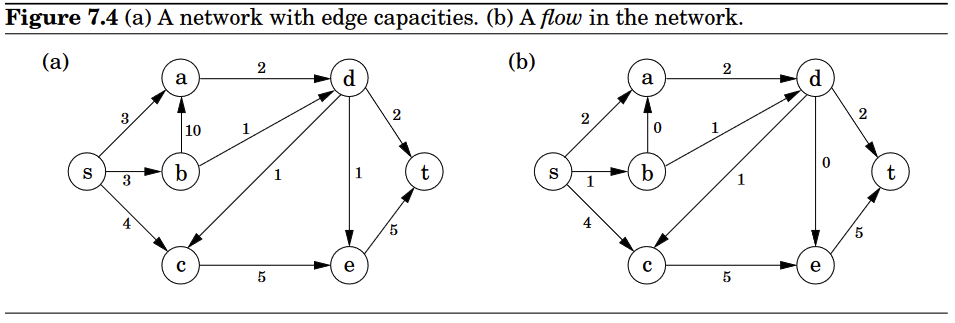
The networks we are dealing with consist of a directed graph ; two special nodes , which are, respectively, a source and sink of G; and capacities on the edges.
We would like to send as much things as possible from to without exceeding the capacities of any of the edges. A particular shipping scheme is called a flow and consists of a variable for each edge of the network, satisfying the following two properties:
- Doesn’t violate edge capacities
- For all nodes except and , the amount of flow entering and the amount of flow leaving should be the same ⇒ flow is conserved
-
The size of a flow is the total quantity sent form to and is the quantity leaving
We can solve max flow by Ford-Fulkerson

- Find an augmenting path in the graph
- BFS(Edmonds–Karp), A* search, RL Model
- Construct the residual graph by augmenting the path based on the original graph and augmenting path
- Do this until no augmenting path can be found.
The max flow problem can also be reduced to a LP problem
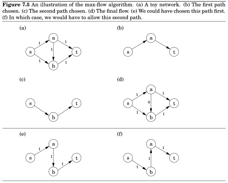
Once we have studied the simplex algorithm in more detail (DPV 7.6), we will be in a position to understand exactly how it handles flow LPs, which is useful as a source of inspiration for designing direct max-flow algorithms. It turns out that in fact the behavior of simplex has an elementary interpretation:
- Start with zero flow.
- Repeat: choose an appropriate path from s to t, and increase flow along the edges of this path as much as possible.
- See Figure 7.5 (a-d) for example
- There is just one complication.
- What if we had initially chosen a different path, the one in Figure 7.5(e)?
- This gives only one unit of flow and yet seems to block all other paths.
- Simplex gets around this problem by also allowing paths to cancel existing flow.
- In this particular case, it would subsequently choose the path of Figure 7.5(f). Edge of this path isn’t in the original network and has the effect of canceling flow previously assigned to edge .
- What if we had initially chosen a different path, the one in Figure 7.5(e)?
in each iteration simplex looks for an path whose edges can be of two types
- is in the original network, and is not yet at full capacity
- The reverse edge is in the original network, and there is some flow along it
If the current flow is f , then in the first case, edge can handle up to additional units of flow, and in the second case, upto fvu additional units (canceling all or part of the existing flow on ). These flow-increasing opportunities can be captured in a residual network , which has exactly the two types of edges listed, with residual capacities :
Thus we can equivalently think of simplex as choosing an path in the residual network
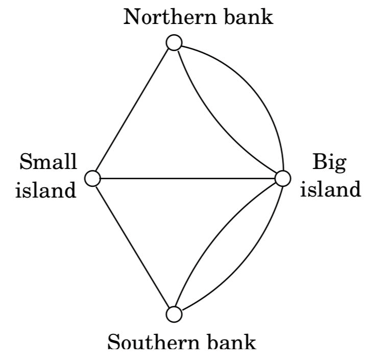
Partition the nodes of the oil network (Figure 7.4) into two groups, and :
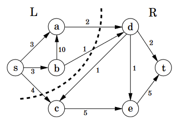
Any oil transmitted must pass from to . Therefore, no flow can possibly exceed the total capacity of the edges from to , which is 7. But this means that the flow we found earlier, of size 7, must be optimal
Some cuts are large and give loose upper bounds— has a capacity of 19. But there is also a cut of capacity 7, which is effectively a certificate of optimality of the maximum flow. Such a cut always exists.
Max-flow min-cut theorem
The size of the maximum flow in a network equals the capacity of the smallest -cut. Moreover, our algorithm automatically finds this cut as a by-product!
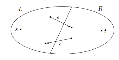
Suppose is the final flow when the algorithm terminates. We know that node is no longer reachable from in the residual network . Let be the nodes that are reachable from in , and let be the rest of the nodes. Then is a cut in the graph G:
We claim that:
Runtime:
Each iteration requires time if a DPS or BPS is used to find an path.
Suppose all edges in the original network have integer capacities . Then an inductive argument shows that on each iteration of the algorithm, the flow is always an integer and increases by an integer amount. Therefore, since the maximum flow is at most ⇒ the number of iterations is at most this much.
But what if is big? However, if paths are chosen in a sensible manner—in particular, by using BFS, which finds the path with the fewest edges—then the number of iterations is at most
Bipartite Matching
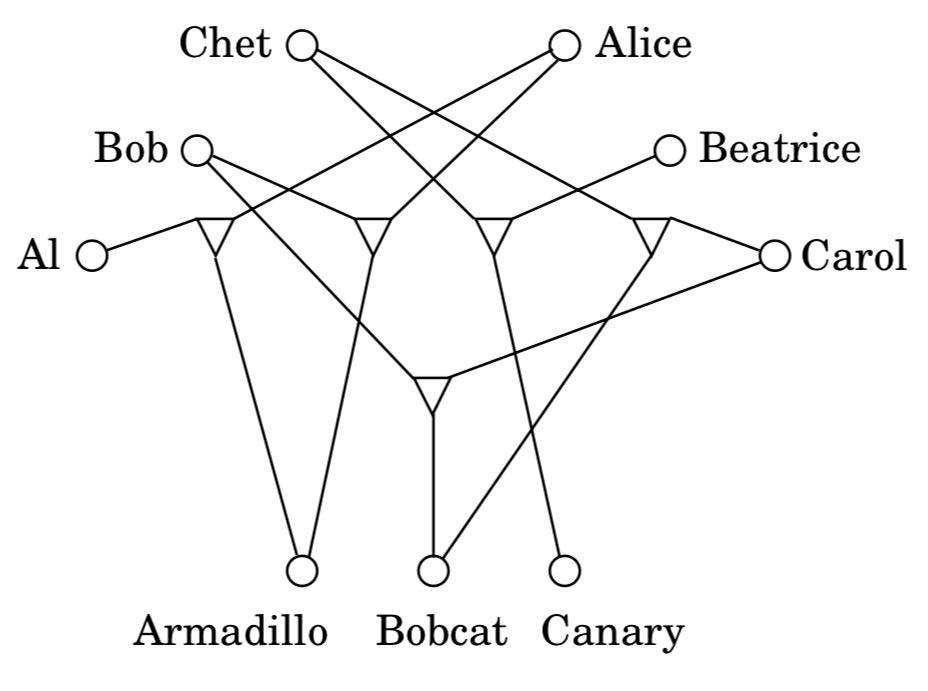
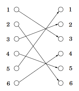
There is an edge between a boy and girl if they like each other (for instance, Al likes all the girls). Is it possible to choose couples so that everyone has exactly one partner, and it is someone they like? In graph-theoretic jargon, is there a perfect matching?
Create a new source node, s, with outgoing edges to all the boys; a new sink node, t, with incoming edges from all the girls; and direct all the edges in the original bipartite graph from boy to girl (Figure 7.8). Finally, give every edge a capacity of 1. Then there is a perfect matching if and only if this network has a flow whose size equals the number of couples.
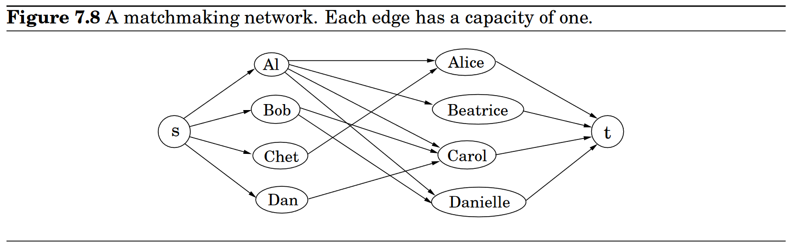
Nice property about max flow problem: if all edge capacities are integers, then the optimal flow found by our algorithm is integral
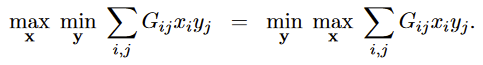
Zero-sum Games (DPV 7.5)
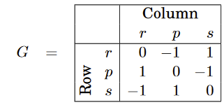
Now suppose the two of them play this game repeatedly. If Row always makes the same move, Column will quickly catch on and will always play the countermove, winning every time. Therefore Row should mix things up: we can model this by allowing Row to have a mixed strategy, in which on each turn she plays with probability , with probability , and with probability . This strategy is specified by the vector . Similarily, Column’s mixed strategy is some .
On any given round of the game, there is an chance that Row and Column will play the i-th and j-th moves, respectively.
Therefore the expected(avergae) gain of Row is:
If we investigate with a nonsymmetric game ⇒ then the “best” each player can do might be different
Imagine a presidential election scenario in which there are two candidates for office, and the moves they make correspond to campaign issues on which they can focus (the initials stand for economy, society, morality, and tax cut). The payoff entries are millions of votes lost by Column.
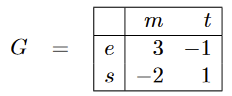
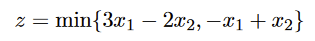
Suppose now Row’s strategy is The objective of Column :
Since Row knows that it is forced to announce its strategy,
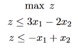
We can transform this problem into an LP:
Dual of this LP: If Column anounces strategy first and then Row chooses
Multiplicative Weights Algorithm / Hedge Algorithm
Per-step regret
Consider the following online optimization setup:
- On each time step we can choose among possible strategies
- we are required to produce a strategy array where and .
- After we make our choice of , a loss array is revealed
- Therefore our loss at time is
-
- The regret at time is defined as
-
-
- We will use to denote all possible probability distributions over elements
-
- We assume that . If losses are in different range, we can scale them and shift them to be between 0 and 1
The algorithm:
- has
- hardcoded in the algorithm
- Maintains a set of weights at each time step
-
-
- Each step,
-
Multiplicative Weights in Minmax Games
- Suppose is the payoff matrix for the fist player
- denotes the probability vector of player 1’s strategy
- denotes the probability vector of player 2’s strategy
- Loss for player 1 is
- Loss for player 2 is
Bounds:
- For both players
-
-
Circuit Evaluation (DPV 7.7)
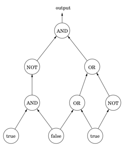
We are given a Boolean circuit, a DAG of gates of the following types
- Input gates have indegree zero, with value true or false
- AND gates and OR gates have indegree 2
- NOT gates have indegree 1
Additionally, one of the gates is designated as the output.
CIRCUIT VALUE problem: apply Boolean logic to the gates in topological order, does the output evaluate to true?
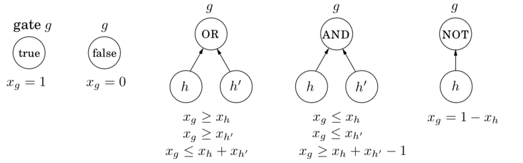
⬆️Additional Constraints imposed by different gates
Those constraints forces each to be (false) or (true).
Turns out the CIRCUIT VALUE problem is the most general problem solvable in polynomial time, every algorithm will eventually run on a computer, and the computer is ultimately a Boolean combinational circuit implemented on a chip. If the algorithm runs in polynomial time, it can be rendered as a Boolean circuit consisting of polynomially many copies of the computer’s circuit, one per unit of time.
Hence, the fact that CIRCUIT VALUE reduces to linear programming means that all problems that can be solved in polynomial time do!
NP-Complete Problems (DPV 8)
Search Problems (DPV8.1)
A search problem is specified by an algorithm that takes two inputs, an instance and a proposed solution , and runs in time polynomial in . We say is a solution to if and only if .
SAT(Satisfiability) problem
Given a Boolean Formula in Conjunctive Normal Form (CNF), which is a collection of clauses each containing of disjunction of several literals(either a Boolean variable or the negation of one), find a satisfying truth assignment.
Horn Formula:
- Special form of SAT problem
- At most one positive literal
- Greedy algorithm (DPV 5.3)
2-literals case:
- Solved by DPV 3.28 by strongly connected components of a particularly constructed graph
- Or another polynomial algorithm (DPV 9)
Traveling salesman problem (TSP)
Given vertices and all distances between them, as well as budget . We want to find a tour, a cycle that passes through every vertex exactly once, of total cost or less (or report that no such tour exists)
In other words (in search problem’s perspective), we want to find a permutation such that when they are toured in this order, the total distance covered is at most :
There’s a budget ⇒ solution to a search problem should be easy to recognize (polynomial checkable).
Euler and Rudrata
Euler’s Bridge problem: Is there a path that visits each edge exactly once?
Or in other words: When can a graph be drawn without lifting the pencil from the paper?
Rudrata’s Cycle problem: Can one visit all the squares of the chessboard, without repeating any square, in one long walk that ends at the starting square and at each step makes a legal knight move?
In other words: Given a graph, find a cycle that visits each vertex exactly once - or report that no such cycle exists ⇒ Oops! Looks similar to TSP!
Cuts and Bisections
Balanced Cut problem: Given a graph with vertices and a budget , partition the vertices into two sets and such that and such that there are at most edges between and
Applications: Clustering (problem of segmenting an image into its constituent components (say, an elephant standing in a grassy with a clear blue sky above) ⇒ Put a node for each pixel and put an edge between nodes whose corresponding pixels are spatially close together and also similar in color.
Integer Linear Programming
We mentioned in DPV 7 that there is a different, polynomial algorithm for linear programming. But the situation changes completely if in addition to specifying a linear objective function and linear inequalities, we also constrain the solution(values for the variables) to be integer.
In order to define a search problem, we define goal (counterpart of budget constraint in maximization problems) Then we have:
Special case of ILP (Zero-one Equations [ZOE]):
- Goal to find a vector of and satisfying
- is matrix with entries
Three-Dimensional Matching
boys, girls and pets, and the compatibilities among them are specified by a set of triples , each containing a boy, a girl, and a pet. We want to find disjoint triples and thereby create harmonious households
Independent set, vertex cover, and clique
Independent Set Problem: Given a graph and an integer , find vertices that are independent (no two of which have an edge between them)
Vertex Cover (Special Case of Set Cover): input is a graph and a budget , find vertices that cover every edge
Set Cover: Given a set and several subsets of it, , along with a budget . Select of subsets so that their union is .
CLIQUE problem: Given a graph and a goal , find a set of vertices such that all possible edges between them are present.
Longest Path: Given a graph with nonnegative edge weights ad two distinguished vertices and , along with a goal , we want to find a path from to with total weight at least .
Knapsack and subset sum
KNAPSACK problem (DPV 6.4, DP solution ): Given integer weights and integer values for items. Also given a weight capacity and goal , find a set of items whose total weight is at most and total value is at least .
UNARY KNAPSACK: KNAPSACK with unary-coded integers ()
SUBSET SUM: Each item’s value is equal to its weight (given in binary), goal is the same as the capacity ⇒ finding a subset of given set of integers that adds up to exactly
NP-Complete Problems (DPV 8.2)
The world is full of search problems, some can be solved efficiently, some seem to be very hard
| Hard Problems (NP-Complete) | Easy Problems (in P) |
| 3 SAT | 2 SAT, HORN SAT |
| Traveling Salesman Problem | Minimum Spanning Tree |
| Longest Path | Shortest Path |
| 3D Matching | Bipartite Matching |
| Knapsack | Unary Knapsack |
| Independent Set | Independent Set on Trees |
| Integer LP | Linear Programming |
| Rudrata Path | Euler Path |
| Balanced Cut | Minimum Cut |
P and NP
Search Problems: There is an efficient checking algorithm that takes input a given input (data specifying the problem) and a potential solution , and outputs iff is a solution to instance in polynomial time .
We denote the class of all search problems by (nondeterministic polynomial time).
We also denote the class of all search problems that can be solved in polynomial time by
if , there’s an efficient method to prove any mathematical statement, thus eliminating the need for mathematicians! ⇒ this is a nice intuition of why , however proving this is extremely difficult.
Reductions in search problems
The problem on the left side of the table are all in some sense - exactly the same problem, except that they are stated in different languages. We will use reductions to show that those problems are the hardest problems in - if even one of them has a polynomial time algorithm, then every problem in has a polynomial time algorithm.
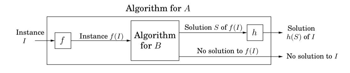
A reduction from search problem to search problem is a polynomial-time algorithm that transforms any instance of into an instance of , together with another polynomial-time algorithm that maps any solution of back into a solution of . If has no solution, then neither does .
Now let’s define the class of hardest search problems
A search problem is NP-complete if all other search problems reduce to it.
Nice properties about reduction:
- Composability
- If , then
- If we proved that is NP-Complete, we just need to show to show that is NP-Complete, because now all problems in NP reduce to .
- If , then
- difficulty flows in the direction of the arrow
- efficient algorithms move in the other direction
A side note on factoring:
Factoring is the task of finding all prime factors of a given integer, but the difficulty of factoring is of a different nature and nobody believes that factoring is NP-complete. One major difference is there’s no scenario such that no solution exists, and the problem succumbs to the power of quantum computation.
The Reductions (DPV 8.3)
Coping with NP-Completeness (DPV 9)
If we have a hard problem
- Start by proving that it is NP-Complete
- A proof by generalization
- Simple reduction from another NP-Complete problem to this problem
- Once problem is proved NP-Complete
- Special cases of the problem might be solved in linear time
- Graph problems can be solved by DP in linear time
- approximation algorithm
- falls short of the optimum but never by too much
- Greedy algorithm for set cover
- heuristics
- algorithms with no guarantees on either the running time or the degree of approximation
- rely on ingenuity, intuition, a good understanding of the application, meticulous experimentation to tackle the problem
Intelligent Exaustive Search (DPV 9.1)
Backtracking
It is often possible to reject a solution by looking at just a small portion of it
By quickly checking and discrediting some partial assignment, we are able to prune some portion of the search space.
Consider the Boolean formula specified by the set of clauses
We will start by branching on any one variable ()
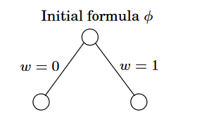
No clause is immediately violated, thus neither of those partial assignments can be eliminated outright. Let’s keep branching on with
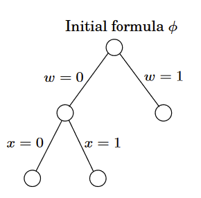
Now we see that violates and this helps us prune a good chunk of search space.
In the case of Boolean satisfiability, each node of the search tree can be described either by a partial assignment or by the clauses that remain when those values are plugged into the original formula.
For instance, if and then any clause with or is instantly satisfied and any literal or is not satisfied and can be removed. What’s left is
Likewise for
“empty clause” rules out satisfiability.
Thus the nodes of the search tree, representing partial assignments, are themselves SAT sub-problems. This alternative representation is helpful for making the two decisions that repeatedly arise: which subproblem to expand next, and which branching variable to use.
Since the benefit of backtracking lies in its ability to eliminate portions of the search space, and since this happens only when an empty clause is encountered, it makes sense to choose the subproblem that contains the smallest clause and to then branch on a variable in that clause.
More abstractly, a backtracking algorithm requires a test that looks like a subproblem and quickly declares one of three outcomes
- Failure: the subproblem has no solution
- Success: A solution to the subproblem is found
- Uncertainty
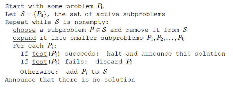
In the case of SAT, this test declares failure if there is an empty clause, success if there are no clauses, and uncertainty otherwise.
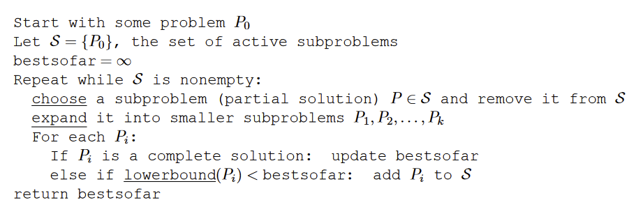
Branch-and-bound
Same principle of backtracing algorithm can be generalized from search problem to optimization problems.
Suppose we have a minimization problem
As before, we need a basis for eliminating partial solutions, since there is no other source of efficiency in our method. To reject a subproblem, we must be certain that its cost exceeds that of some other solution we have already encountered. But its exact cost is unknown to us and is generally not efficiently computable. So instead we use a quick lower bound on this cost.
Use this on TSP problem with graph with edge lengths :
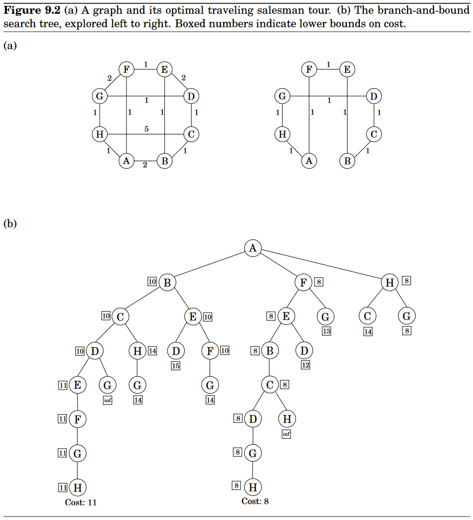
- A partial solution is a simple path passing through some vertices , where includes the endpoints and .
- We can denote such a partial solution by where is fixed throughout the algorithm
- Corresponding subproblem is to find the best completion of the tour (cheapest complementary path with intermediate nodes )
- Initial problem is
- At each step we extend a particular partial solution by a single edge , where
- up to ways to do this
- leads to a subproblem of
- To impose a lower-bound on completing a partial tour , many methods have been proposed, but we can look at some easy ideas:
- Remaining vertices are , plus edges from and to , therefore its cost is at least the sum of
- Lightest edge from to
- Lightest edge from to
- Minimum Spanning Tree of
- Remaining vertices are , plus edges from and to , therefore its cost is at least the sum of
Approximation Algorithms (DPV 9.2)
Suppose we have an algorithm for our problem which given the instance returns a solution with value , the approximation ratio of algorithm is defined as
measures by the factor by which the output of algorithm exceeds the optimal solution, on the worst-case input.
When faced with an NP-complete optimization problem, a reasonable goal is to look for an approximation algorithm whose is as small as possible.
Vertex Cover
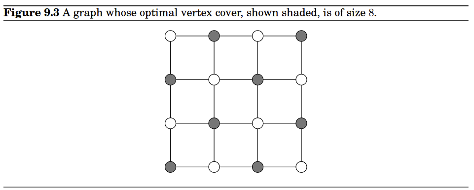
Given an undirected graph , find a subset of the vertices that touches every edge and is minimized.
- A special case of SET COVER
- From DPV 5.4, we know it can be approximated with a factor of by greedy
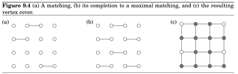
Matching: A subset of edges have no vertices in common are matched together. A matching is maximal if no more edges can be added to it.
any vertex cover of a graph must be at least as large as the number of edges in any matching in ; that is, any matching provides a lower bound on OPT. Simply because each edge of the matching must be covered by one of its endpoints in any vertex cover
let be a set that contains both endpoints of each edge in a maximal matching . Then must be a vertex cover—if it isn’t, that is, if it doesn’t touch some edge , then could not possibly be maximal since we could still add to it. But our cover has vertices. And from the previous paragraph we know that any vertex cover must have size at least , so we are done ( is our approximation of vertex cover)!
This simple procedure always returns a vertex cover whose size is at most twice optimal!
Clustering
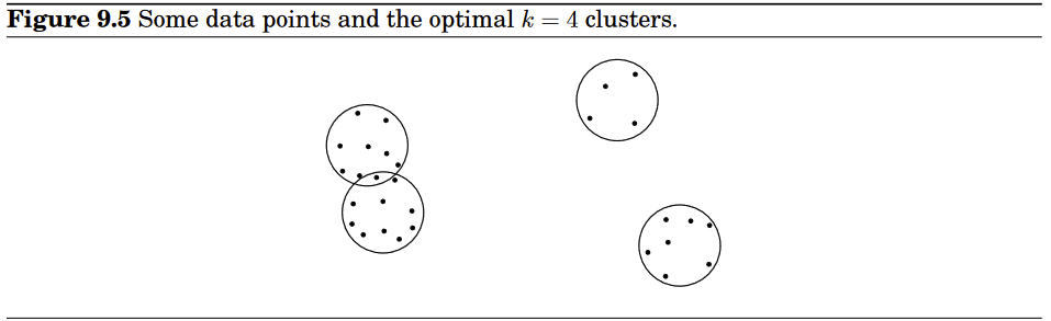
We have some data thaty we want to divide into groups ⇒ first define the notion of “distance”, which has to satisfy the usual “metric” properties
- for all
- iff
-
-
- Triangle inequality
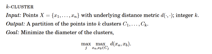
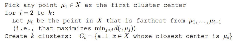
The problem is NP-hard, but there’s an approximation algorithm:
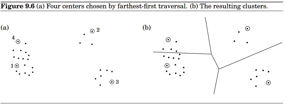
- Pick of data points as cluster centers, assign each of the reamining points to the center closest to it, creating clusters
- Centers picked one at a time, rule: always pick the next center to be as far as possible from the centers chosen so far
Let be the point farthest from (in other words the next center we would have chosen, if we wanted of them), and let be its distance to its closest center. Then every point in must be within distance of its cluster center. By triangular inequality, this means every cluster has diameter at most .
we have identified points that are all at a distance at least from each other ⇒ Any partition into clusters must put two of these points in the same cluster and must therefore have diameter at least .
TSP
We saw that the triangle inequality helped making the k-CLUSTER problem approximable; In TRAVELLING SALESMAN PROBLEM, if the distances between cities satisfy the metric properties, then there is an algorithm that outputs a tour of length at most times optimal. We will look at a weaker result that achieves a factor of .
Is there a structure that is easy to compute and plausibly related to the best traveling salesman tour? Turns out to be the minimum spanning tree.
Removing any edge from a traveling salesman tour leaves a path through all the vertices, with is a spanning tree, therefore
Now a MST is not necessarily a tour. In order to make this a tour, try use each edge twice, then follow the shape of the MST we end up with a tour that visits all the cities, some of them more than once.
Therefore this tour has a length at most twice the MST cost
To fix the problem of visiting some cities more than once, the tour should simply skip any city it is about to revisit, and instead move directly to the next new city in its list (By the triangle inequality, these bypasses can only make the overall tour shorter).
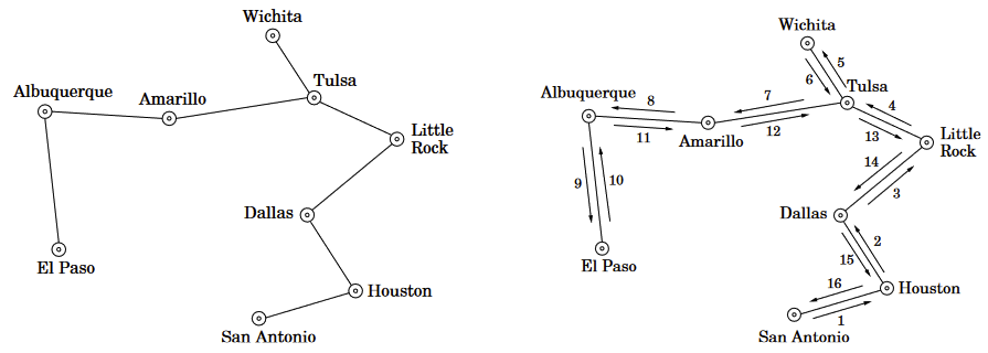
General TSP
Much harder to approximate if TSP does not satisfy the triangle inequality!
Recall that we have a polynomial-time reduction from TSP instance:
- If has a Rudrata path, then , the number of vertices in .
- If has no Rudrata path, then
This means even an approximate solution to TSP would enable us to solve RUDRATA PATH!
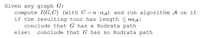
So unless , there cannot exist an efficient approximation algorithm for the general TSP.
Knapsack
This approximation: Given any , it will return a solution of value at least times the optimal value, in time it only scales polynomially in input size and in .
We earlier have a solution to the Knapsack problem with . Using a similar technique, a running time of can also be achived. Neither of those running times is polynomial because and can be very larger, exponential in size of the input.
Let’s consider the algorithm. In the bad case when is large, what if we simply scale down all the values in some way?
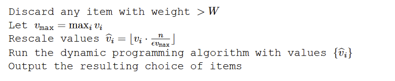
Let’s see why this works. First of all, since the rescaled values are all at most , the dynamic program is efficient, running in time .
Now suppose the optimal solution to the original problem is to pick some subset of items , with total value , the rescaled value of this same assignment is
Therefore the optimal assignment for the shrunken problem, call it , has a rescaled value of at least this much. In terms of the original values, assignment has a value of at least
The approximability hierarchy
NP-Complete optimization problems are classified as follows (assuming , if then all classes collapse into one):
- Those of which like TSP, no finite approximation ratio is possible
- Those for which an approximation ratio is possible, but there are limits to how small this can be
- Vertex Cover, k-Cluster, TSP with triangle inequality
- Those for which approximability has no limits, and polynomial approximation algorithms with error ratios arbitrarily close to zero exist.
- Knapsack
- Those for which the approximation ratio is about
- Set Cover
Local Search Heuristics (DPV 9.3)
For minimization problem, “try out” local solutions, keep them if they work well
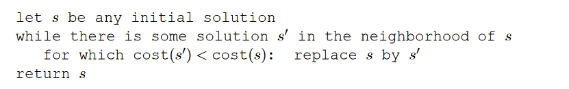
On each iteration, the current solution is replaced by a better one close to it, in its neighborhood. This neighborhood structure is something we impose upon the problem and is the central design decision in local search.
TSP with local search
Assume we have all interpoint distances between cities, giving a search space of different tours. What is a good notion of neighborhood?
- Define two tours as being close if they only differ in a few edges
- They cannot differ in just one edge (cuz we have to include every vertices)
- So we will consider differences of two edges
- We define the 2-change neighborhood of tour s as being the set of tours that can be obtained by removing two edges of s and then putting in two other edges.
- It is quick because a tour only has neighbours
- But unclear how many iterations will be needed
- But the final answer is only lcocally optimal
- We can fix by making it a 3-change, or 4-change, etc. But each iteration is more expensive now
Graph Partitioning
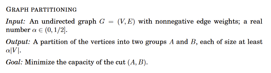
Removing the restriction on the sizes of and would give the MINIMUM CUT problem, which can be efficiently solved using flow techniques.
However, this present variant is NP-hard.
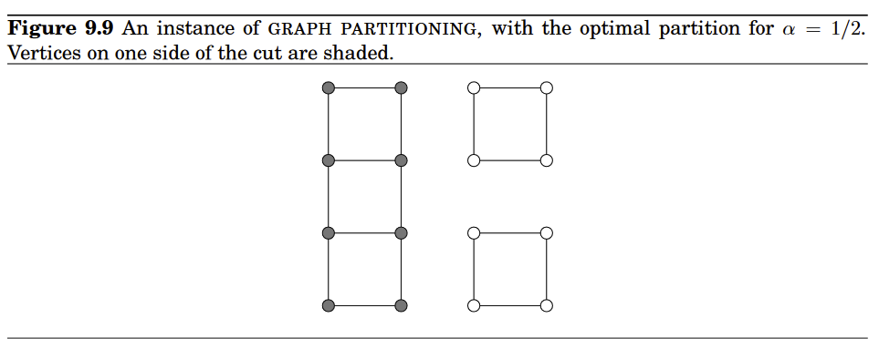
Let with be a candidate solution; We will define its neighbors to be all solutions obtainable by swapping one pair of vertices across the cut: all solutions of the form where .
How do we improve local search procedures?
Dealing with Local Optima
Randomization and restarts
Randomization
- Invaluable ally in local search
- Used to
- pick a random initial solution
- choose a local move when several are available
When there are many local optima, randomization is a way of making sure that there is at least some probability of getting to the right one.
Simulated Annealing
As the problem size grows, the ratio of bad to good local optima often increases, sometimes to the point of being exponentially large. In such cases, simply repeating the local search a few times is ineffective.
- What about we occasionally allow moves that actually increase the cost, in the hope that they will pull the search out of dead ends?
- The method of simulated annealing redefines the local search by introducing the notion of a temperature .
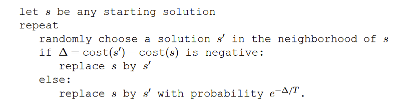
- Trick is to start with large and gradually reduce it to zero
- it is quite an art to choose a good timetable by which to decrease the temperature, called an annealing schedule.
Randomized Algorithms
We now study randomized algorithms instead of a deterministic algorithm. A randomized algorithm can be seen as a regular algorithm but takes two inputs: usual input and uniformly random string for some . We generally categorize randomized algorithms into two classes
- Las Vegas
- Algorithms for which correctness guarentees
- Runtime with input with randomness is a random variable
- Then we talk about being the expected runtime of on inputs of size
-
- e.g. Quicksort worst case is but expectation is
- Monte Carlo
- Runtime is always bounded by some desired bound
- but correctness is a random variable
- Let be the “indicator random variable” for the event that returns an incorrect value ( when is incorrect and otherwise.
-
Primality Testing (DPV 1.3)
Is there some test that tells us whether a number is prime without factoring out the number?
Fermat’s Little Theorem (assuming is prime)
Proof:
Let be the nonzero integers modulo ; that is, . One crucial observation: the effect of multiplying these numbers by a (modulo p) is simply to permute them.
Let’s expand this equivalence to a set
If we multiply everything in the set together,
Divide by on each side, we get exactly Fermat’s Little Theorem
We’ll prove that when the elements of S are multiplied by modulo , the resulting numbers are all distinct and nonzero. And since they lie in the range [1, p − 1], they must simply be a permutation of S.
The numbers are distinct because if , then dividing both sides
by a gives .
They are nonzero because similarly implies . (And we can divide by , because by assumption it is nonzero and therefore relatively prime to )
Therefore we can write
Multiply each element in
Dividing by (which we can do because it is relatively prime to p, since p is assumed prime) then gives the theorem.
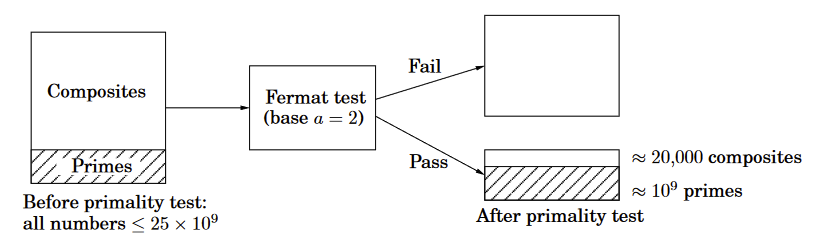
So Fermat’s theorem suggests a “factorless” test
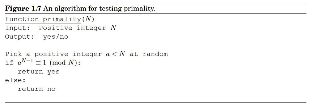
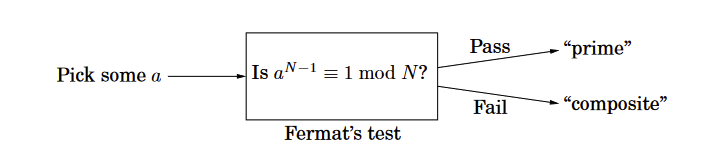
The problem is that Fermat’s theorem is not an if-and-only-if condition; it doesn’t say what happens when N is not prime, so in these cases the preceding diagram is questionable. In fact, it is possible for a composite number N to pass Fermat’s test (that is, ) for certain choices of .
It turns out that certain extremely rare composite numbers N , called Carmichael numbers, pass Fermat’s test for all relatively prime to . On such numbers our algorithm will fail; but they are pathologically rare, and we will later see how to deal with them.
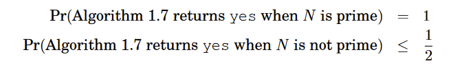
We will ignore those Carmichael numbers for now; We will show that fails Fermat’s test for at least half of the possible values of
Lemma: If for some relatively prime to , then it must hold for at least half the choices of .
Proof: Fix some value of for which , the key is to notice that every element that passes Fermat’s test with respect to has a twin, that fails the test:
Moreover, all these elements , for fixed but different choices of , are distinct, for the same reason in the proof of Fermat’s test: just divide by .
The one-to-one function shows that at least as many elements fail the test as pass it
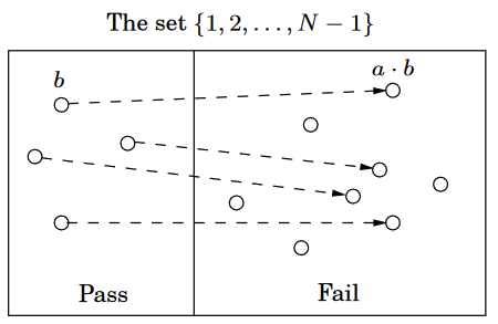
Therefore the algorithm in Figure 1.7 has the following property
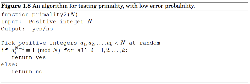
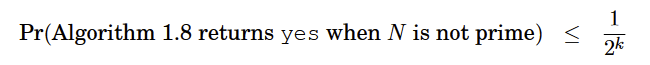
Generating Random Primes
Let be the number of primes , then , more precisely
Such abundance makes it simple to generate a random n-bit prime:
- Pick a random n-bit number
- Run a primality test on
- If it passes the test, output , otherwise repeat the process
Chamichael numbers
The smallest Carmichael number is , it is not a prime; Yet it fools the fermat test because for all values of relatively prime to . For a long time it was thought that there might be only finitely many numbers of this type, but we know that they are infinite, but exceedingly rare.
There is a way around Carmichael numbers, using a slightly more refined primality test due to Rabin and Miller.
Write in the form , we will choose a random base and check the value of . Perform this computation by first determining and then repeatedly squaring, to get the sequence:
If , then is composite by Fermat’s little theorem, and we’re done. If , we conduct a little follow-up test
- Somewhere in the preceeding sequence, we ran into a 1 for the first time.
- If this happened after the first position (if ) and the preceeding value in the value in the list is not , then we declare composite
- we have found a nontrivial square root of 1 modulo N : a number that is not ±1 mod N but that when squared is equal to 1 mod N
- Such a number can only exist if is composite
Quicksort
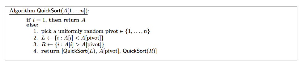
The key insight is that the runtime is, up to a constant factor, equal to the number of comparisons performed by QuickSort.
This is because for every recursive call on some array of size, say, , the total time spent at that level of recursion (steps 1 through 3 above) is , whereas the number of comparisons is also .
Furthermore, for any pair of indices , is compared to either or times throughout the entire run of the algorithm; this is because for two items to be compared, one of them had to have been the pivot, in which case the non-pivot item is then put into either L or R and never has a chance to be compared with the pivot again.
Thus if we define an indicator random variable which is if the i-th smallest element is ever compared with the j-th smallest and otherwise, we have that
where is a constant
Applying linearity of expectation,
Let’s try to bound
What is the probability that the ith and jth smallest elements (call them ) are ever compared? If we trace the QuickSort recursion tree from the root, both elements start off being in the same recursive subproblem, then when the root recursion node picks a random pivot, if that pivot is either or then and either both go to or both go to (i.e. stay in the same recursive subproblem). Otherwise, if the pivot is in , then they do not go to the same recursive subproblem.
Thus what decides whether equals 0 or 1 is the following: it is equal to 1 iff the first time a pivot is picked in the set S, it is picked to be either or ; otherwise since will be sent separately to and and never have a chance to be compared again. Thus .
Doing some algebraic manipulation
We proved expected runtime, but can we prove that the runtime is low with high probability?
Recall Markov’s inequality (With as a nonnegative random variable)
Therefore for runtime of QuickSort, , since is nonnegative (algorithms cannot run in negative time), we can apply Markov’s inequality, . Thus the runtime is 99% probability within
Freivalds’ Algorithm
How do we verify computation correctness?
Freivalds’ algorithm specifically focuses on verifying matrix-matrix multiplication. That is, we have two matrices and would like to know . We could of course multiply these matrices ourselves in time (or faster using Strassen or more recent algorithms), but if we upload to the cloud which returns some to us, is there a way to verify that much faster than doing the multiplication ourselves from scratch?
Answer is yes using randomization: pick a uniformly random and check whether .
Claim: If , then , otherwise
Proof:
For the second half (assuming ), let’s define
Then and in particular its ith column is nonzero for some .
Now suppose for some particular , , then if but the i-th entry flipped, we have since , where is the i-th standard basis vector.
Now let’s pair all the elements of into pairs, where each pair differs in only the i-th entry. Then we see that in each pair at most one of or can equal zero, but not both. Thus , leading to the probability for the second half.
If we want to reduce our probability of returning an incorrect answer to some desired failure probability , we can for example set and pick random vectors independently. We then declare iff , then the probability we fail is at most . Our runtime would be .
Karger’s Global Minimum Cut Algorithm (Contraction Algorithm)
Given a (possibly weighted) undireced graph and we would like to find a cut of smallest size. A cut is a partition of the vertices into two non-empty sets .
The size of the cut is defined to be . If unweighted it would be .
For Contraction algorithm we will focus only on unweighted case (but it is possible to adapt the algorithm to the weighted case as well). Assuming the graph is connected ( because otherwise we can find a cut of size using DFS or BFS by having be one connected component and be everything else)
First note that maximum flow can be used to solve global mincut deterministically. But global minimum cut has to seperate vertex from some other vertex , though we do not know a priori which one, thus set and loop over all possibilities for . For each possibility we compute the min-cut as discused in earlier lectures. In an unweighted graph the capacities are all so the value of max flow / min cut is at most . Thus eaach min-cut computation takes using Ford-Fulkerson. Since we do s-t mincut computations, the total time is .
We now analyze Karger’s simpler Contraction algorithm,
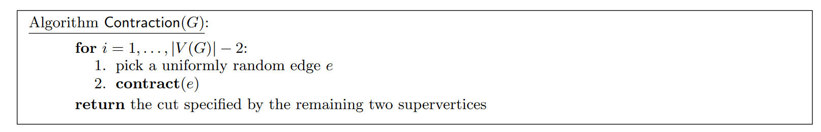
The contract operation on
- Removes from the graph and adds a new merged “supervertex” into the graph
- All edges used to point into either or now point into
- If a vertex had edges to both and , then both edges remain and both point to
- Thus the algorithm can create multi-edges
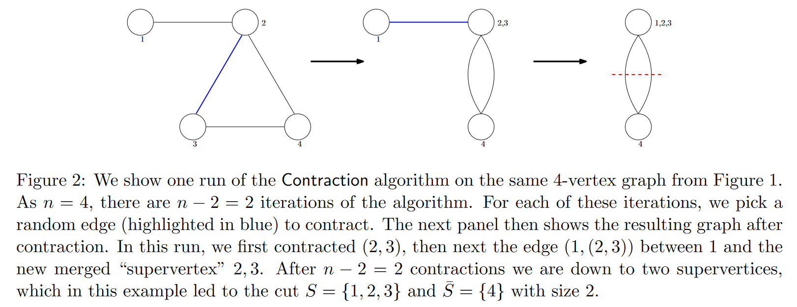
Lemma: For an graph , fix a particular global minimum cut , then the probability that return this particular cut is at least
Proof:
The contraction algorithm algorithm will return iff no edge crossing the cut is ever contracted. Let be the number of edges crossing the cut, and let and denote the number of edges and corresponding vertices in the graph during the ith iteration of the for loop, ( is just and is a random variable that depends on what has been contracted so far, then the probability we never contract an edge crossing this cut is precisely
Now we get a handle on the , contracting an edge cannot decrease the minimum cut value. Thus for each intermediate graph throughout the run of the algorithm, the minimum cut value is always
In the ith iteration , but we just argued that
Thus
Therefore we can plug that into our product formula and get
This also implies that any graph has at most minimum cuts.
This is in fact tight: the cycle on vertices has exactly global min-cuts: pick an arbitrary two edges to cut and let be the two distinct arcs that are disconnected by removing those two edges.
Furthermore, it is possible to implemenet the Contraction algorithm in time, but we will not give the details here.
However, the bound given by the Lemma seems a bit problematic: we want a bigger probability larger than , so can we do better than that?
We run the algorithm times independently return the smallest cut ever found. To analyze this, we make use of the follwoing useful fact from calculus, using convexity of the function .
Fact 5: For all
Proof: Define . Taylor’s theorem gives for some . But note that for all , so therefore , thus
Probability that we will never find a global min cut is at most (with repeating the algorithm times)
Overall runtime is to succeed with probability . Comparable to max flow based approach using Ford-Fulkerson (though we have a factor), but is much simpler
Streaming Algorithms
- Make one pass over large dataset to support future queries
- We want a very low-memory data structure
- Dynamic data structures
Types of problems
- Counting problems
- graph problems
- find a path
- frequency-based problems
Counter
init():
	N = 0

incr():
	N++

query():
	return N
Takes bits
Can we do better?
Approximate Counting
Can we remember the exponent instead of the actual number?
And now we only need to take bits, which is
What if instead of using a base of 2, we use a base of ?
Note: If , then
Therefore to remember , it takes around
But how would we increment since we don’t know ?
incr(), With chance , we increment
LEMMA: Let be the value of after calls to incr(), then
Proof (by induction on ):
base case:
So therefore we return when query() is called.
But what about the error? We can bound
Where
Optimal choice:
Randomized Counting
init():
	X = 0

incr():
	if rand() is even:
		X++

query():
	return 2X
Distinct Counting
Return number of distinct elements in stream that consist of ints picked from
Hashed Distinct Counting
- Pick random hash function
- Assume is independent and uniformly random
- Initiate
- For each in stream,
-
-
- For each in stream,
- when
query(): return
- Keep smallest hash values
-
-
- when
query(), return
- Memory grows linearly with
Industry standard: Hyperloglog
Lower bounds
Prove that any algorithm for existing problem has to take time
Time Hierarchy Theorem (CS172)
For any , problmes requiring time.
e.g.
Circuit Complexity
Boolean circuit made up of AND, OR, NOT, each gate taking two inputs and having one output, and input bits
Since standard computation model algorithm ⇒ efficient circuits,
lower bounds on circuits ⇒ LBs on standard algorithms
But what does “efficient circuit” mean? Can it be quantified?
- circuit sizes : # of wires
- # circuits of size is
- # functions is
- Vast majority to problems need large circuits ⇒ large runtime
- There exists an explicit problem requiring circuits of size (2016)
- Depth of the circuit
Uniform Circuits:
s.t. spits out efficiently
Multiplication
Spectral Graph Theory
Unserstanding properties of graph by looking at eigenvalues/eigenvectors of associated matrices
example:
(1) adjacency matrix
(2) Graph Laplacian
⇒ degree of vertex (# of edges connected to )
“unnomralized laplacian”
We also have “normalized laplacian”
Random Walks
Do steps of random walk from vertex
Let be the standard basis vector for vertex
Basically, having means we’re definitely at vertex
Say go from some probability distribution on to in one random walk step
We see:
So
Note:
We can use this to calculate the cost of having a cut